Steps to generate models#
This notebook outlines steps for generating the pre-computed models provided with Dustapprox.
The process typically involves the following steps:
download or provide atmosphere models
select extinction curves
select passbands to compute extinction in
Generate a grid of models for various values of \(A_0\) and \(R_0\) (or other extinction curve parameters)
Fit polynomial models to the extinction values as a function of \(A_0\), \(R_0\), and commonly \(T_{eff}\) or colors.
Export the models to ECSV files for later use.
version
This notebook is based on Dustapprox version 0.2.0.
Warning
This process can be computationally intensive and may take some time to complete.
Intermediate data not provided
We do not provide the intermediate data files (e.g., the atmosphere models or the full grid of extinction values before fitting) due to their large size. However, the code provided here allows you to reproduce the models if needed.
# import package or add to path from source
try:
    import dustapprox
except ImportError:
    import sys
    sys.path.insert(0, "../src")
    import dustapprox
%matplotlib inline
import matplotlib.pyplot as plt
Available extinction curves#
Dusapprox uses dust_extinction as provider of dust extinction curves. Fig. 8 shows some of the available extinction curves. Not all extinction curves are suitable for all applications, weavelength ranges, parameters, etc vary between curves. We primarily use the parametric average average curves here, but you can always manually use a different one. Please refer to the dust_extinction documentation for more details.
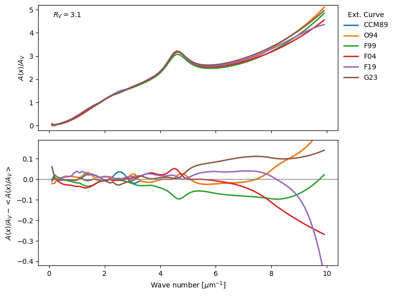
Fig. 8 Comparison of several extinction curves. Top: Extinction curves normalized to their parameter A\(_V\). Bottom: Difference to the mean extinction curve to emphasize the variations. The curves are computed for the parameter R\(_V\)=3.1.#
See also
Available passbands#
For the photometry, we use pyphot a suite to compute synthetic photometry in flexible ways.
Using pyphot v2.0.0
For more information about pyphot, and the internal photometric computations, please refer to its documentation.
Through the SVO Profile Service#
dustapprox.io.svo.get_svo_passbands() is a wrapper around pyphot to interface the SVO Filter Profile Service, which provides us with a large collection of passbands. Fig. 9 shows an example of passbands retrieved from the SVO service.
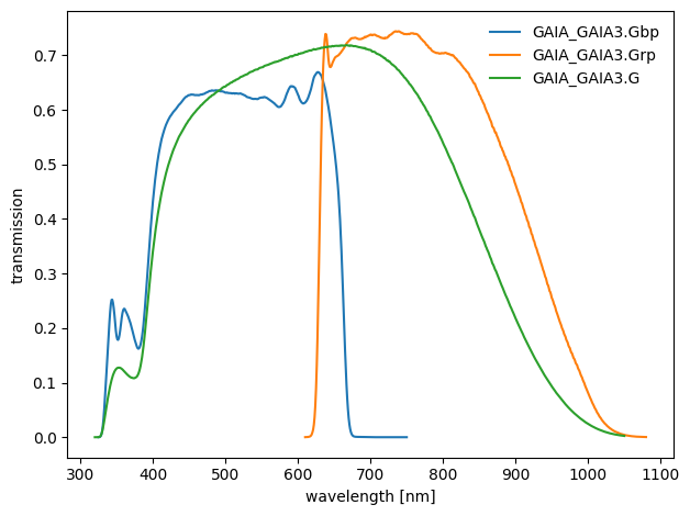
Fig. 9 Gaia eDR3 passbands retrieved from the SVO service.#
Passbands from local ascii files#
Pyphot also provides all features to read passbands from local ascii files. Fig. 10 shows an example of the Gaia C1 passbands (Jordi et al 2006) read from dustapprox distributed ascii files. The C1B and C1M systems for the broad and medium band passbands, respectively. The C1 system was specifically designed to maximize the scientific return in terms of stellar astrophysical parameters, but was not implemented in favor of the Gaia BP/RP prism spectra.

Fig. 10 Gaia C1 passbands from dustapprox provided ascii files. The Broad passbands are shown in full strength, while the medium ones are shown at half strength for clarity.#
Generating the pre-computed models#
Warning
This process can be computationally intensive and may take some time to complete.
define the set of filters you want to compute the models for.#
Here is an example of some commonly used sets of filters:
# List of common sets of filters we use to generate pre-computed models for dustapprox.

gaia_filters = ['GAIA/GAIA3.G', 'GAIA/GAIA3.Gbp', 'GAIA/GAIA3.Grp',]
sloan_filters = ['SLOAN/SDSS.u', 'SLOAN/SDSS.g', 'SLOAN/SDSS.r', 'SLOAN/SDSS.i', 'SLOAN/SDSS.z',]
twomass_filters = ['2MASS/2MASS.J', '2MASS/2MASS.H', '2MASS/2MASS.Ks',]
wise_filters = ['WISE/WISE.W1', 'WISE/WISE.W2', 'WISE/WISE.W3', 'WISE/WISE.W4',]
galex_filters = ['GALEX/GALEX.FUV', 'GALEX/GALEX.NUV',]
generic_filters = ['Generic/Johnson.U', 'Generic/Johnson.B', 'Generic/Johnson.V',
                   'Generic/Cousins.R', 'Generic/Cousins.I',
                   'Generic/Bessell_JHKLM.J', 'Generic/Bessell_JHKLM.H', 'Generic/Bessell_JHKLM.K',]
In the following, we will use the Gaia filters gaia_filters as an example.
Define the atmosphere models.#
As internally we calculate the relative change in flux of the spectra, we do not need absolute flux-calibrated models and use the atmospheres directly (i.e. no rescaling with radius or bolometric luminosity). Here we use the Kurucz 2003 models taken from the SVO Theoretical spectra service. These models span ranges of from 3,500 K to 50,000 K, from 0 to 5 dex, and metallicity from -4 to 0 dex. Our approach is agnostics to the exact library itself. All files from SVO have the same format, but the spectra are not on the same wavelength scale (even for a single atmosphere source). The parameters of the spectra may vary from source to source. For instance, they may not provide microturbulence velocity or [\(\alpha\)/Fe] etc. We technically require only effective temperature and surface gravity to be provided.
See also
Atmosphere models for further information and download links to some precompiled atmospheres.
The following code snippet shows how to generate the pre-computed models using the generate_grid() function from dustapprox.tools.generate_model module. It is basically a loop over the model atmosphere files, the A0 and R0 values, and the selected filters.
The internal function generate_grid() handles all the details of reading the atmosphere models, applying the extinction curves, computing synthetic photometry, and exporting the results to ECSV files. It also allows parallel processing through joblib to speed up the computation.
from dustapprox.tools import generate_model
import pathlib

# features = 'teff logg feh A0 alpha'.split()
features = "teff A0 R0".split()
model_pattern = "models/Kurucz2003all/*.fl.dat.txt"
# model_pattern = "../docs/models/Kurucz2003all/*.fl.dat.txt"
name = gaia_filters[0].split("/")[0].lower()
output_path = pathlib.Path(f"precomputed/grids/kurucz_{name}_f99_a0r0_grid.ecsv")
atmosphere_name = "Kurucz (ODFNEW/NOVER 2003)"
extinction_curve = "F99"

# Compute the grid -- this may take a while -- reuses existing grids if available
r = generate_model.generate_grid(
    model_pattern,
    output_path,
    gaia_filters,
    atmosphere_name=atmosphere_name,
    extinction_curve=extinction_curve,
    n_jobs=-1
)
Computing photometric grid
   - Using passbands: GAIA/GAIA3.G, GAIA/GAIA3.Gbp, GAIA/GAIA3.Grp
   - Using model pattern: models/Kurucz2003all/*.fl.dat.txt
   - Using atmospheres: Kurucz (ODFNEW/NOVER 2003)
   - Using extinction curve: F99
   - Using default A0 values: [0.01, 0.1, 0.2 ... 20.0]
   - Using default R0 values: [2.3, 2.6, 3.1, 3.6, 4.1, 4.6, 5.1]
   - Using default parameters: ('teff', 'logg', 'feh', 'alpha')
Exporting grid to precomputed/grids/kurucz_gaia_f99_a0r0_grid.ecsv. Done.
Note
Saving files as ECSV ensures compatibility with any platform that can read ascii files. ECSV preserves metadata, such as column names and data types, which is essential for later use.
For photometric grids, this generates large files that could benefit from other formats. However, these are intermediate files that we do not provide with dustapprox.
Train and export the polynomial models#
The final step involves fitting polynomial models to the computed extinction values as a function of \(A_0\), potentially \(R_0\), and other parameters like \(T_{eff}\). This is done using the dustapprox.tools.generate_model.train_polynomial_model() module, which fits the polynomials, and provides means to export the fitted models to new ECSV files for later use in dustapprox. A wrapper function dustapprox.tools.generate_model.export_trained_model_to_ecsv() is provided to handle the entire process in one go.
For this step, we define what features are used in the polynomial fitting. In our case, we will use teff, A0, and R0.
Note
The choice of features depends on the specific application and the desired accuracy of the extinction models. Including more features can improve the fit but may also increase the complexity of the models.
features = "teff A0 R0".split()
atmosphere_shortname = 'kurucz'
force_recompute = False    # Change here to True to force recomputing the model
model_output_path = pathlib.Path(
        f"precomputed/polynomial/{extinction_curve}/{atmosphere_shortname}/{name}_{atmosphere_shortname}_{extinction_curve}_{'_'.join(features).lower()}.ecsv"
    )
if model_output_path.exists() and not force_recompute:
    print(f"Model file {model_output_path} already exists. Skipping model fitting.")
else:
    if not force_recompute:
        print(f"Model file {model_output_path} does not exist. Fitting model.")
    else:
        print(f"Forced recomputing is True. Fitting model.")
        models = generate_model.train_polynomial_model(r, model_output_path, features, degree=3)
        generate_model.export_trained_model_to_ecsv(model_output_path, models)
Model file precomputed/polynomial/F99/kurucz/gaia_kurucz_F99_teff_a0_r0.ecsv already exists. Skipping model fitting.
The models are exported as ECSV files for later use with dustapprox.
Reloading precomputed models#
We use dustapprox.models.PrecomputedModel to define our library and its find() method to search available models and associated passbands.
The search can be on passband, extinction, atmosphere, and model kind. It is caseless and does not need to contain the complete name.
import pathlib
from dustapprox.models import PrecomputedModel

features = "teff A0 R0".split()
atmosphere_shortname = 'kurucz'
extinction_curve = "F99"
name = "gaia"
force_recompute = True
model_output_path = pathlib.Path(
        f"precomputed/polynomial/{extinction_curve}/{atmosphere_shortname}/{name}_{atmosphere_shortname}_{extinction_curve}_{'_'.join(features).lower()}.ecsv"
    )

lib = PrecomputedModel(str(model_output_path.parent))
lib.get_models_info()
[]
a = lib.find(passband='GAIA3.Gbp', extinction='F99', atmosphere='kurucz', kind='polynomial')[0]
a.load_model()
[PolynomialModel: None
 <dustapprox.models.polynomial.PolynomialModel object at 0x1120b20c0>
    from: A0, R0, teffnorm   polynomial degree: 3]
Shortcuts with dustapprox.tools.generate_model module#
To simplify the process of generating grids and fitting models, dustapprox provides the dustapprox.tools.generate_model module and the dustapprox.tools.generate_model.main_example() function. This module encapsulates the entire workflow into convenient classes and functions.
from dustapprox.tools.generate_model import GridParameters, train_polynomial_model, gaia_dr3_filters
import numpy as np
import pathlib

def main_example():
    """Generate a pre-computed polynomial model library end-to-end"""

    name = "gaia"
    features = ["teff", "A0", "R0"]

    # helps to robustly define grid parameters
    grid_parameters = GridParameters(
        model_pattern="models/Kurucz2003all/*.fl.dat.txt",
        pbset=gaia_dr3_filters,
        atmosphere_name="Kurucz (ODFNEW/NOVER 2003)",
        atmosphere_shortname="kurucz",
        extinction_curve="F99",
        apfields=("teff", "logg", "feh", "alpha"),  # no additional output parameters
        n_jobs=-1,
        A0=np.sort(np.hstack([[0.01], np.arange(0.1, 20.01, 0.1)])),
        R0=np.array([2.3, 2.6, 3.1, 3.6, 4.1, 4.6, 5.1]),
    )

    grid_output_path = pathlib.Path(
        f"precomputed/grids/{name}_{grid_parameters.atmosphere_shortname}_{grid_parameters.extinction_curve}_grid.ecsv"
    )

    # run grid generation
    grid = grid_parameters.generate_grid(grid_output_path)

    # Train models on the generated grid
    model_output_path = pathlib.Path(
        f"precomputed/polynomial/{grid_parameters.extinction_curve}/{grid_parameters.atmosphere_shortname}/{name}_{grid_parameters.atmosphere_shortname}_{grid_parameters.extinction_curve}_{'_'.join(features)}.ecsv"
    )
    model_kwargs = {"degree": 3}

    train_polynomial_model(grid, model_output_path, features, **model_kwargs)

    lib = PrecomputedModel(str(model_output_path.parent))
    return lib
The GridParameters dataclass allows you to specify all the parameters needed to generate the grid, while the generate_grid() method handles the actual computation.
The train_polynomial_model() function fits the polynomial models and saves them to the specified output path.
Running full model generation#
Important
To be added
List all available models#
The following shows how to list all available pre-computed models in the dustapprox library.
import pandas as pd
from dustapprox.models import PrecomputedModel

lib = PrecomputedModel()

data_ = []
for info in lib.get_models_info():

    kind = info.model['kind']
    features = ' '.join(info.model['feature_names'])
    extc = info.extinction['source']
    atm = info.extinction['source']
    teffmin = info.atmosphere['teff'][0]
    teffmax = info.atmosphere['teff'][1]
    loggmin = info.atmosphere['logg'][0]
    loggmax = info.atmosphere['logg'][1]
    fehmin = info.atmosphere['feh'][0]
    fehmax = info.atmosphere['feh'][1]
    a0min = info.extinction['A0'][0]
    a0max = info.extinction['A0'][1]
    if 'R0' in info.extinction:
            r0min = info.extinction['R0'][0]
            r0max = info.extinction['R0'][1]
    else:
        r0min, r0max = 3.1, 3.1

    if kind == 'polynomial':
        kind = "{kind:s}(degree={degree:d})".format(kind=kind,
                                                    degree=info.model['degree'])

    for pb in info.passbands:
        data_.append([pb, kind, features,
                     extc, a0min, a0max, r0min, r0max,
                     atm, teffmin, teffmax, loggmin, loggmax, fehmin, fehmax])
columns=['passband', 'kind', 'features',
         'extinction', 'A0 min', 'A0 max', 'R0 min', 'R0 max',
         'atmosphere', 'teff min', 'teff max', 'logg min', 'logg max',
         '[Fe/H] min', '[Fe/H] max']

pd.DataFrame.from_records(data_, columns=columns).set_index('passband').sort_index().head()
| kind | features | extinction | A0 min | A0 max | R0 min | R0 max | atmosphere | teff min | teff max | logg min | logg max | [Fe/H] min | [Fe/H] max | |
|---|---|---|---|---|---|---|---|---|---|---|---|---|---|---|
| passband | ||||||||||||||
| 2MASS_2MASS.H | polynomial(degree=3) | A0 teffnorm | Fitzpatrick (1999) | 0.01 | 20.0 | 3.1 | 3.1 | Fitzpatrick (1999) | 3500.0 | 50000.0 | 0.0 | 5.0 | -4.0 | 0.5 |
| 2MASS_2MASS.H | polynomial(degree=3) | A0 R0 teffnorm | F99 | 0.01 | 20.0 | 2.3 | 5.1 | F99 | 3500.0 | 50000.0 | 0.0 | 5.0 | -4.0 | 0.5 |
| 2MASS_2MASS.J | polynomial(degree=3) | A0 teffnorm | Fitzpatrick (1999) | 0.01 | 20.0 | 3.1 | 3.1 | Fitzpatrick (1999) | 3500.0 | 50000.0 | 0.0 | 5.0 | -4.0 | 0.5 |
| 2MASS_2MASS.J | polynomial(degree=3) | A0 R0 teffnorm | F99 | 0.01 | 20.0 | 2.3 | 5.1 | F99 | 3500.0 | 50000.0 | 0.0 | 5.0 | -4.0 | 0.5 |
| 2MASS_2MASS.Ks | polynomial(degree=3) | A0 teffnorm | Fitzpatrick (1999) | 0.01 | 20.0 | 3.1 | 3.1 | Fitzpatrick (1999) | 3500.0 | 50000.0 | 0.0 | 5.0 | -4.0 | 0.5 |
See also
Extinction approximation models for the complete list.
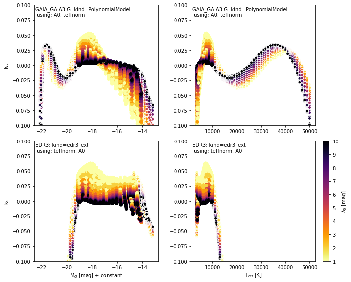
Comparing with EDR3 extinction#
We provide the EDR3 model from Riello et al. (2020) (module-dustapprox.literature.edr3. They fit a similar polynomial equation on a grid of extinctions obtained by convolving the Gaia eDR3 passbands with Kurucz spectra (Castelli & Kurucz, 2003) and the
Fitzpatrick et al. (2019) extinction curve. They constructed a grid with \(3500 K < T_{eff}
< 10000 K\) in steps of \(250 K\), and \(0.01 < A_0 < 20 mag\) with a step linearly
increasing with \(0.01 mag\)
from dustapprox.literature import edr3
edr3ext = edr3.edr3_ext()
kg_bab = edr3ext.from_teff('kG', df['teff'], df['A0'])
delta_edr3 = df['mag'] - df['A0'] * kg_bab - df['mag0']
ydata = (df['mag'] - df['mag0']) / df['A0']
ypred = model.predict(df)
delta = df['mag'] - df['A0'] * ypred - df['mag0']

from sklearn.metrics import mean_absolute_error, root_mean_squared_error
stats = {'mean': np.mean, 'std': np.std,
         'mae': lambda x: mean_absolute_error(x, np.zeros_like(x)),
         'rmse': lambda x: root_mean_squared_error(x, np.zeros_like(x))}


selection = 'A0 > 0.0'
select = df.eval(selection)
print(f"""Our model ({selection})""")
[print("    ", sname, '=', sk(ydata[select] - ypred[select])) for sname, sk in stats.items()]
print(f"""EDR3 model ({selection})""")
[print("    ", sname, '=', sk(ydata[select] - kg_bab[select])) for sname, sk in stats.items()]

selection = '3500 < teff < 10_000'
select = df.eval(selection)
print(f"""\nOur model ({selection})""")
[print("    ", sname, '=', sk(ydata[select] - ypred[select])) for sname, sk in stats.items()]
print(f"""EDR3 model ({selection})""")
[print("    ", sname, '=', sk(ydata[select] - kg_bab[select])) for sname, sk in stats.items()];
Our model (A0 > 0.0)
     mean = -1.2335793396269397e-14
     std = 0.006371610131284496
     mae = 0.004285260812386554
     rmse = 0.006371610131284496
EDR3 model (A0 > 0.0)
     mean = -2.6226363805751904
     std = 7.01279579721422
     mae = 2.6226363805751904
     rmse = 7.487157436446889

Our model (3500 < teff < 10_000)
     mean = 0.0022291703821189636
     std = 0.005015272890195844
     mae = 0.00430507292284872
     rmse = 0.005488366128061226
EDR3 model (3500 < teff < 10_000)
     mean = -0.1560191806864705
     std = 0.05344416757431945
     mae = 0.1560191806864705
     rmse = 0.16491896128034964
import pandas as pd
from dustapprox import models
from dustapprox.literature import edr3
import pylab as plt

# get Gaia models
lib = models.PrecomputedModel()
# r_ = lib.find(passband='Gaia')[0]  # taking the first one
model = lib.load_model('../gaiadr3_a0_tmp.ecsv', passband='GAIA_GAIA3.G')

# get some data
data = pd.read_csv('../docs/models/precomputed/kurucz_gaiaedr3_small_a0_grid.csv')
df = data[(data['passband'] == 'GAIA_GAIA3.G') & (data['A0'] > 0)]

# values
ydata = (df['mag'] - df['mag0']) / df['A0']
kg_edr3 = edr3.edr3_ext().from_teff('kG', df['teff'], df['A0'])
delta_edr3 = ydata - kg_edr3
delta = ydata - model.predict(df)
# note: edr3 model valid for 3500 < teff < 10_000
selection = '3500 < teff < 10_000'
select = df.eval(selection)

plt.figure(figsize=(10, 8))
cmap = plt.cm.inferno_r

title = "{name:s}: kind={kind:s}\n using: {features}".format(
        name=model.name,
        kind=model.__class__.__name__,
        features=', '.join(model.feature_names))

kwargs_all = dict(rasterized=True, edgecolor='w', cmap=cmap, c=df['A0'])
kwargs_select = dict(rasterized=True, cmap=cmap, c=df['A0'][select])

ax0 = plt.subplot(221)
plt.scatter(df['mag0'], delta, **kwargs_all)
plt.scatter(df['mag0'][select], delta[select], **kwargs_select)
plt.colorbar().set_label(r'A$_0$ [mag]')
plt.ylabel(r'k$_G$')
plt.text(0.01, 0.99, title, fontsize='medium',
        transform=plt.gca().transAxes, va='top', ha='left')

ax1 = plt.subplot(222, sharey=ax0)
plt.scatter(df['teff'], delta, **kwargs_all)
plt.scatter(df['teff'][select], delta[select], **kwargs_select)
plt.colorbar().set_label(r'A$_0$ [mag]')
plt.text(0.01, 0.99, title, fontsize='medium',
        transform=plt.gca().transAxes, va='top', ha='left')

title = "{name:s}: kind={kind:s}\n using: {features}".format(
           name="EDR3",
           kind=edr3.edr3_ext().__class__.__name__,
           features=', '.join(('teffnorm', 'A0')))

ax = plt.subplot(223, sharex=ax0, sharey=ax0)
plt.scatter(df['mag0'], delta_edr3, **kwargs_all)
plt.scatter(df['mag0'][select], delta_edr3[select], **kwargs_select)
plt.colorbar().set_label(r'A$_0$ [mag]')
plt.xlabel(r'M$_G$ [mag] + constant')
plt.ylabel(r'k$_G$')
plt.ylim(-0.1, 0.1)
plt.text(0.01, 0.99, title, fontsize='medium',
        transform=plt.gca().transAxes, va='top', ha='left')


plt.subplot(224, sharex=ax1, sharey=ax1)
plt.scatter(df['teff'], delta_edr3, **kwargs_all)
plt.scatter(df['teff'][select], delta_edr3[select], **kwargs_select)
plt.xlabel(r'T$_{\rm eff}$ [K]')
plt.colorbar().set_label(r'A$_0$ [mag]')
plt.ylim(-0.1, 0.1)

plt.setp(plt.gcf().get_axes()[1:-1:2], visible=False)

plt.text(0.01, 0.99, title, fontsize='medium',
        transform=plt.gca().transAxes, va='top', ha='left')

plt.tight_layout()
See also
dustapprox.literature for other literature models.
Assessing models accuracy and systematics for more details.