Extinction curves

In our application, we need the models that predict spectra or SEDs of star extinguished by dust. Interstellar dust extinguishes stellar light as it travels from the star’s surface to the observer. The wavelength dependence of the extinction from the ultraviolet to the near-infrared has been measured along many sightlines in the Milky Way (Cardelli et al. 1989; Fitzpatrick 1999; Valencic et al. 2004; Gordon et al. 2009) and for a handful of sightlines in the Magellanic Clouds (Gordon & Clayton 1998; Misselt et al. 1999; Maiz Apellaniz & Rubio 2012) as well as in M31 (Bianchi et al. 1996, Clayton et al. 2015).

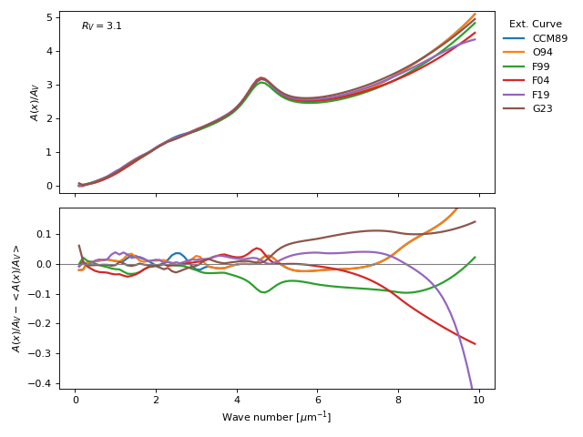
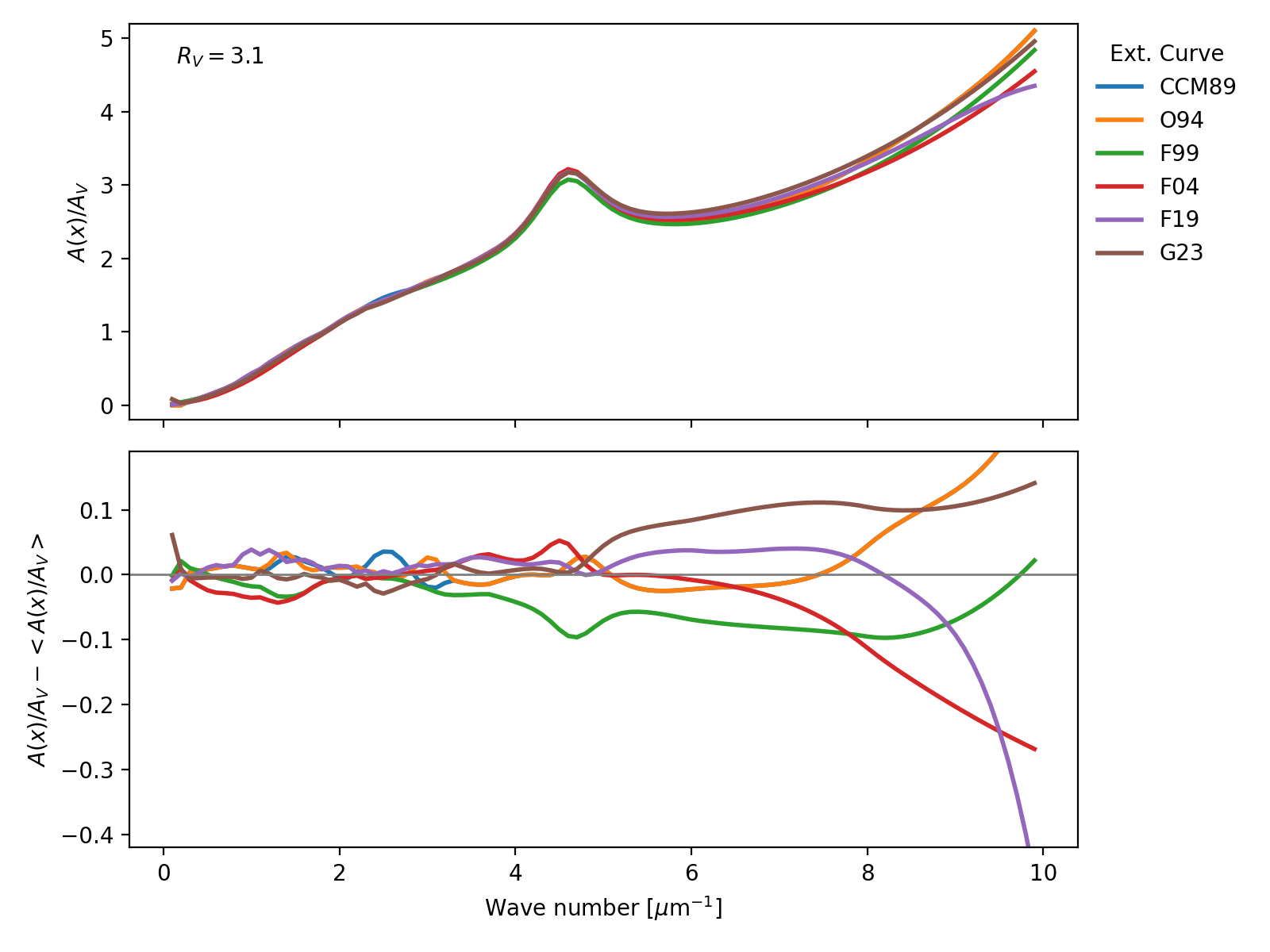
Since v.0.20, Dusapprox uses dust_extinction as provider of dust extinction curves. The following figure shows some of the available extinction curves. Not all extinction curves are suitable for all applications, wavelength ranges, parameters, etc vary between curves. We primarily use the parametric average average curves here, but you can always manually use a different one. Please refer to the dust_extinction documentation for more details.

import numpy as np
import matplotlib.pyplot as plt
import astropy.units as u

from dustapprox.extinction import evaluate_extinction_model

#define the wave numbers
x = np.arange(0.1, 10, 0.1)    # in microns^{-1}
λ = 1. / x * u.micron

curves = 'CCM89', 'O94', 'F99', 'F04', 'F19', 'G23'
R0 = 3.1

curve_data = {}
_, axes = plt.subplots(2, 1, figsize=(8, 6), sharex=True)
for name in curves:
    values = evaluate_extinction_model(name, λ, A0=1.0, R0=R0)
    curve_data[name] = values
    axes[0].plot(x, values, label=f'{name:s}', lw=2)

mean_curve = np.nanmean(list(curve_data.values()), axis=0)
for name, values in curve_data.items():
    diff = values - mean_curve
    axes[1].plot(x, diff, label=f'{name:s}', lw=2)

axes[0].set_ylabel(r'$A(x)/A_V$')
axes[0].legend(loc='upper left', frameon=False, title=rf'Ext. Curve', bbox_to_anchor=(1.0, 1.0))
axes[0].text(0.05, 0.9, rf'$R_V={R0:.1f}$', transform=axes[0].transAxes)
axes[1].set_xlabel(r'Wave number [$\mu$m$^{-1}$]')
axes[1].set_ylabel(r'$A(x)/A_V - <A(x)/A_V>$')
axes[1].axhline(0.0, color='0.5', ls='-', lw=1)
axes[0].set_ylim(-0.2, 5.2)
axes[1].set_ylim(-0.42, 0.19)
plt.tight_layout()
plt.show()

(Source code, png, hires.png, pdf)

Fig. 4 Figure 4. Differences between extinction curves. This figure compares a few different presscriptions at fixed \(R_0\).