dustapprox package#

Submodules#

dustapprox.extinction module#

Dust Extinction curves#

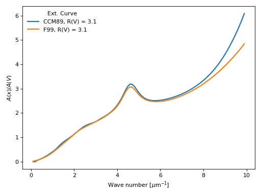
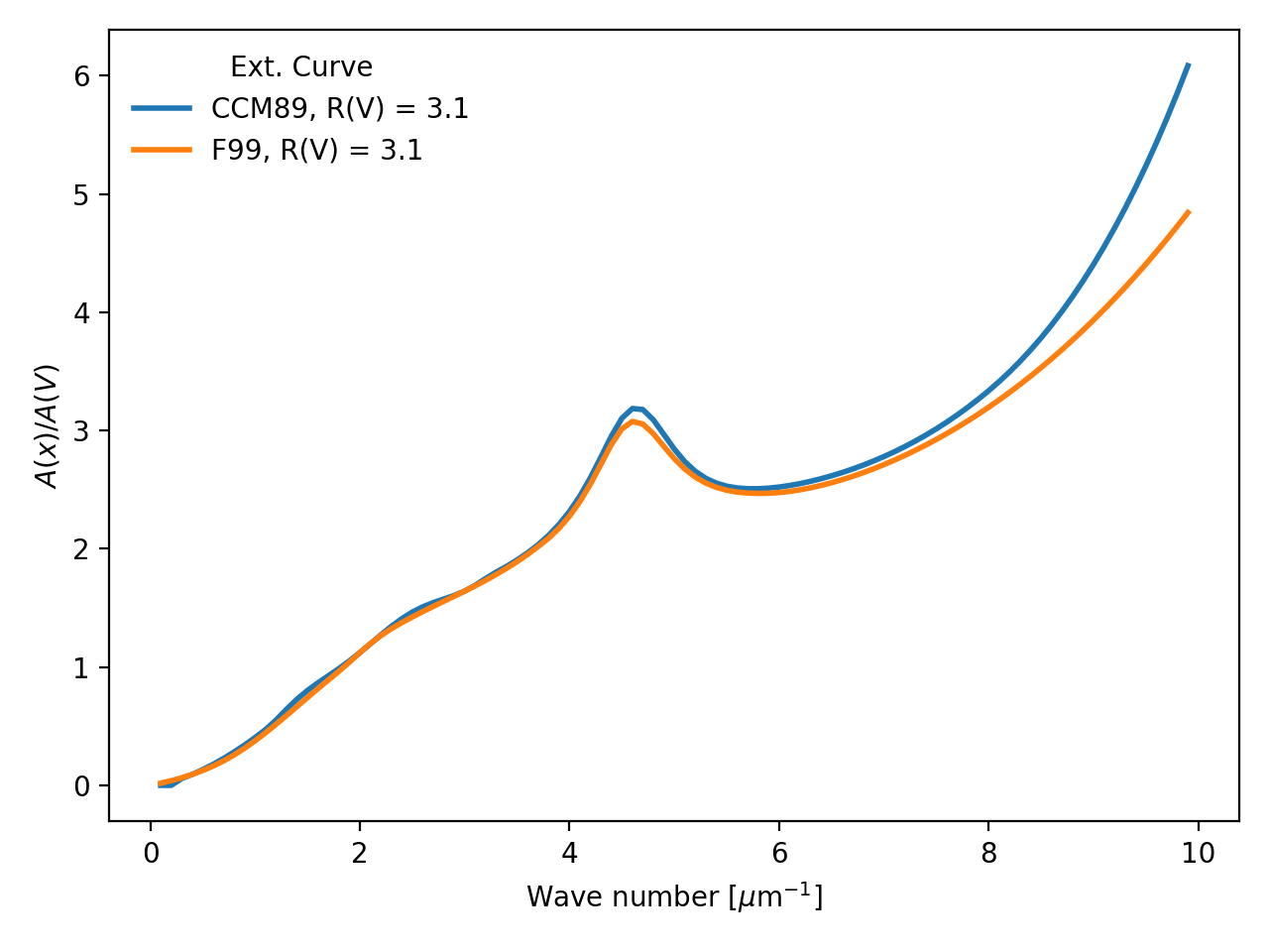
The observations show a wide range of dust column normalized extinction curves, \(A(\lambda) / A(V)\). This package provides a common interface to many commonly used extinction curves.

Note

This module is able to handle values with units from pyphot.astropy (intefaced to this package) and astropy. We recommend the users to provide units in their inputs.

Example of comparing extinction curves

import numpy as np
import matplotlib.pyplot as plt
import astropy.units as u

from dustapprox.extinction import CCM89, F99

#define the wave numbers
x = np.arange(0.1, 10, 0.1)    # in microns^{-1}
lamb = 1. / x * u.micron

curves = [CCM89(), F99()]
Rv = 3.1

for c in curves:
    name = c.name
    plt.plot(x, c(lamb, Rv=Rv), label=f'{name:s}, R(V) = {Rv:0.1f}', lw=2)
plt.xlabel(r'Wave number [$\mu$m$^{-1}$]')
plt.ylabel(r'$A(x)/A(V)$')
plt.legend(loc='upper left', frameon=False, title='Ext. Curve')
plt.tight_layout()
plt.show()

(Source code, png, hires.png, pdf)

class dustapprox.extinction.CCM89[source]#

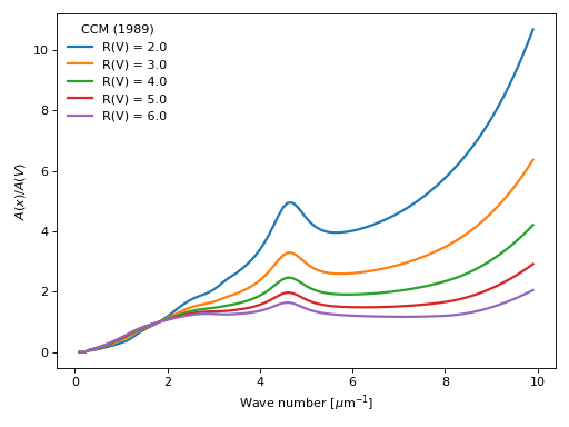
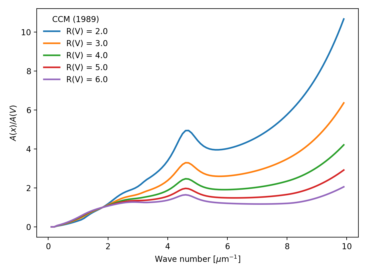
Bases: dustapprox.extinction.ExtinctionLaw

Cardelli, Clayton, & Mathis (1989) Milky Way R(V) dependent model.

from Cardelli, Clayton, and Mathis (1989, ApJ, 345, 245)

Example showing CCM89 curves for a range of R(V) values.

import numpy as np
import matplotlib.pyplot as plt
import astropy.units as u

from dustapprox.extinction import CCM89

#define the wave numbers
x = np.arange(0.1, 10, 0.1)    # in microns^{-1}
lamb = 1. / x * u.micron

c = CCM89()
Rvs = np.arange(2, 6.01, 1.)

for Rv in Rvs:
    plt.plot(x, c(lamb, Rv=Rv), label=f'R(V) = {Rv:0.1f}', lw=2)
plt.xlabel(r'Wave number [$\mu$m$^{-1}$]')
plt.ylabel(r'$A(x)/A(V)$')
plt.legend(loc='upper left', frameon=False, title='CCM (1989)')
plt.tight_layout()
plt.show()

(Source code, png, hires.png, pdf)

class dustapprox.extinction.ExtinctionLaw[source]#

Bases: object

Template function class

name#

name of the curve

Type: str

Parameters: lamb (float, np.array, Quantity) – wavelength. User should prefer a Quantity which provides units.
Returns: val – expected values of the law evaluated at lamb
Return type: ndarray

isvalid(*args, **kwargs)[source]#: Check if the current arguments are in the validity domain of the law Must be redefined if any restriction applies to the law

class dustapprox.extinction.F99[source]#

Bases: dustapprox.extinction.ExtinctionLaw

Fitzpatrick (1999, PASP, 111, 63) [1999PASP..111…63F]_

R(V) dependent extinction curve that explicitly deals with optical/NIR extinction being measured from broad/medium band photometry. Based on fm_unred.pro from the IDL astronomy library

Parameters

lamb (float or ndarray(dtype=float) or Quantity) – wavelength at which evaluate the law. units are assumed to be Angstroms if not provided
Av (float, optional) – desired A(V) (default 1.0)
Rv (float, optional) – desired R(V) (default 3.1)
Alambda (bool, optional) – if set returns +2.5*1./log(10.)*tau, tau otherwise

Returns

r – attenuation as a function of wavelength depending on Alambda option +2.5*1./log(10.)*tau, or tau

Return type

float or ndarray(dtype=float)

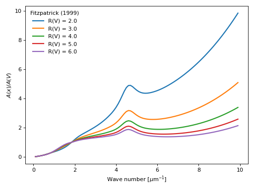
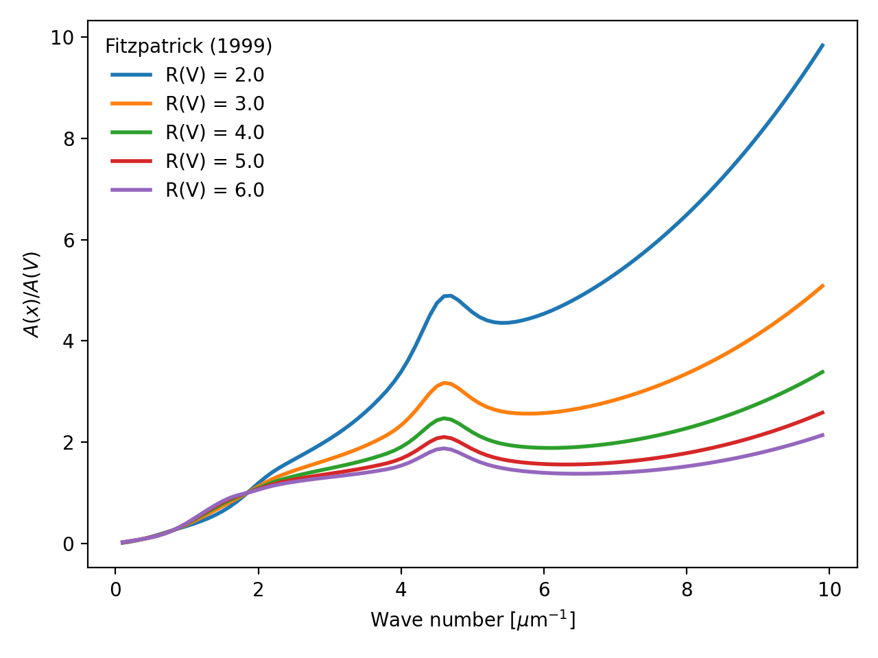
Example showing F99 curves for a range of R(V) values.

import numpy as np
import matplotlib.pyplot as plt
import astropy.units as u

from dustapprox.extinction import F99

#define the wave numbers
x = np.arange(0.1, 10, 0.1)    # in microns^{-1}
lamb = 1. / x * u.micron

c = F99()
Rvs = np.arange(2, 6.01, 1.)

for Rv in Rvs:
    plt.plot(x, c(lamb, Rv=Rv), label=f'R(V) = {Rv:0.1f}', lw=2)
plt.xlabel(r'Wave number [$\mu$m$^{-1}$]')
plt.ylabel(r'$A(x)/A(V)$')
plt.legend(loc='upper left', frameon=False, title='Fitzpatrick (1999)')
plt.tight_layout()
plt.show()

(Source code, png, hires.png, pdf)

Note

this function assumed the wavelength in Anstroms if lamb is not a Quantity.

dustapprox

dustapprox package

Contents

dustapprox package#

Subpackages#

Submodules#

dustapprox.extinction module#

Dust Extinction curves#

dustapprox.version module#