dustapprox.models package

We provide various modeling schemes for extinction in a given photometric band.

Todo

• add script to generate grid of models

• add polynomial training.

• compare literature values to ours.

class dustapprox.models.PrecomputedModel(location=None)

Bases: object

Access to precomputed models

from dustapprox.models import PrecomputedModel
lib = PrecomputedModel()
# search for GALEX passbands if present
r = lib.find(passband='galex')
print(r)
# load both available models
models = []
for source in r.values():
    models.extend([lib.load_model(r, passband=pbname) for pbname in source['passbands']])

result from PrecomputedModel.find()

[{'atmosphere': {'source': 'Kurucz (ODFNEW/NOVER 2003)',
    'teff': [3500.0, 50000.0],
    'logg': [0.0, 5.0],
    'feh': [-4, 0.5],
    'alpha': [0, 0.4]},
  'extinction': {'source': 'Fitzpatrick (1999)', 'R0': 3.1, 'A0': [0, 10]},
  'comment': ['teffnorm = teff / 5040', 'predicts kx = Ax / A0'],
  'model': {'kind': 'polynomial',
  'degree': 3,
  'interaction_only': False,
  'include_bias': True,
  'feature_names': ['A0', 'teffnorm']},
  'passbands': ['GALEX_GALEX.FUV', 'GALEX_GALEX.NUV'],
  'filename': 'dustapprox/data/precomputed/polynomial/f99/kurucz/kurucz_f99_a0_teff.ecsv'}]

result when loading models with from PrecomputedModel.load_model()

[PolynomialModel: GALEX_GALEX.FUV
<dustapprox.models.polynomial.PolynomialModel object at 0x12917b6a0>
    from: A0, teffnorm   polynomial degree: 3,
PolynomialModel: GALEX_GALEX.NUV
<dustapprox.models.polynomial.PolynomialModel object at 0x129170820>
    from: A0, teffnorm   polynomial degree: 3]

find(passband=None, extinction=None, atmosphere=None, kind=None) → Sequence[dict]

Find all the computed models that match the given parameters.

The search is case insentive and returns all matches.

Parameters

• passband (str) – The passband to be used.

• extinction (str) – The extinction model to be used. (e.g., ‘Fitzpatrick’)

• atmosphere (str) – The atmosphere model to be used. (e.g., ‘kurucz’)

• kind (str) – The kind of model to be used (e.g., polynomial).

get_models_info(glob_pattern='/**/*.ecsv') → Sequence[dict]

Retrieve the information for all models available and files

load_model(fname: Union[str, dict], passband: Optional[str] = None)

Load a model from a file or description (PrecomputedModel.find())

Parameters

• fname (str or dict) – The filename of the model to be loaded or a description of the model returned by PrecomputedModel.find()

• passband (str) – The passband to be loaded. If None, loads all available passband models.

Returns

model

Return type

dustapprox.models.polynomial.PolynomialModel

Submodules

dustapprox.models.basemodel module

Base class for deriving various kinds of models.

dustapprox.models.polynomial module

Polynomial approximation of extinction effect per passband.

In this library, we provide tools and pre-computed models to obtain the extinction coefficient \(k_x = A_x / A_0\) for various passbands.

Extinction coefficients depend primarily on the source spectral energy distribution and on the extinction itself (e.g., Gordon et al., 2016; Jordi et al., 2010) but also other parameters such as \(\log g\), \([\alpha/Fe]\), and \([Fe/H]\).

We define the extinction coefficient \(k_x\) as

\[k_x = A_x / A_0,\]

with \(A_0\) the extinction parameter at \(550 nm\), and \(x\) the passband.

We use a L1-regularized regression model (Lasso-Lars model) using BIC or AIC for model/complexity selection.

The optimization objective for Lasso is:

\[\frac{1}{2 n_{samples}} \cdot \|y - X \cdot w\|^2_2 + \alpha \times \|w\|_1\]

AIC is the Akaike information criterion and BIC is the Bayes Information criterion. AIC or BIC are useful criteria to select the value of the regularization parameter \(\alpha\) by making a trade-off between the goodness-of-fit and the complexity of the model.

This allows is to follow the principle of parsimony (aka Occam’s razor): a good model should explain well the data while being simple.

(Source code)

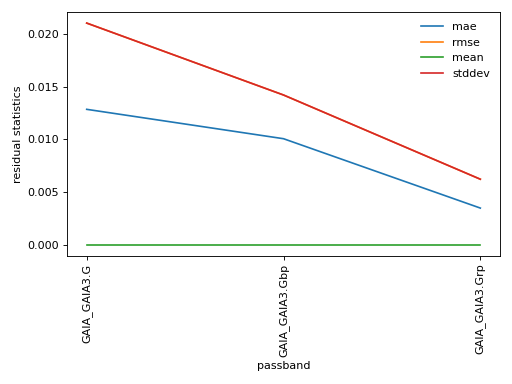
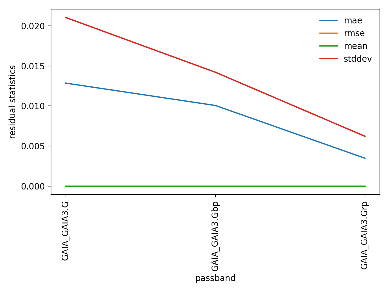
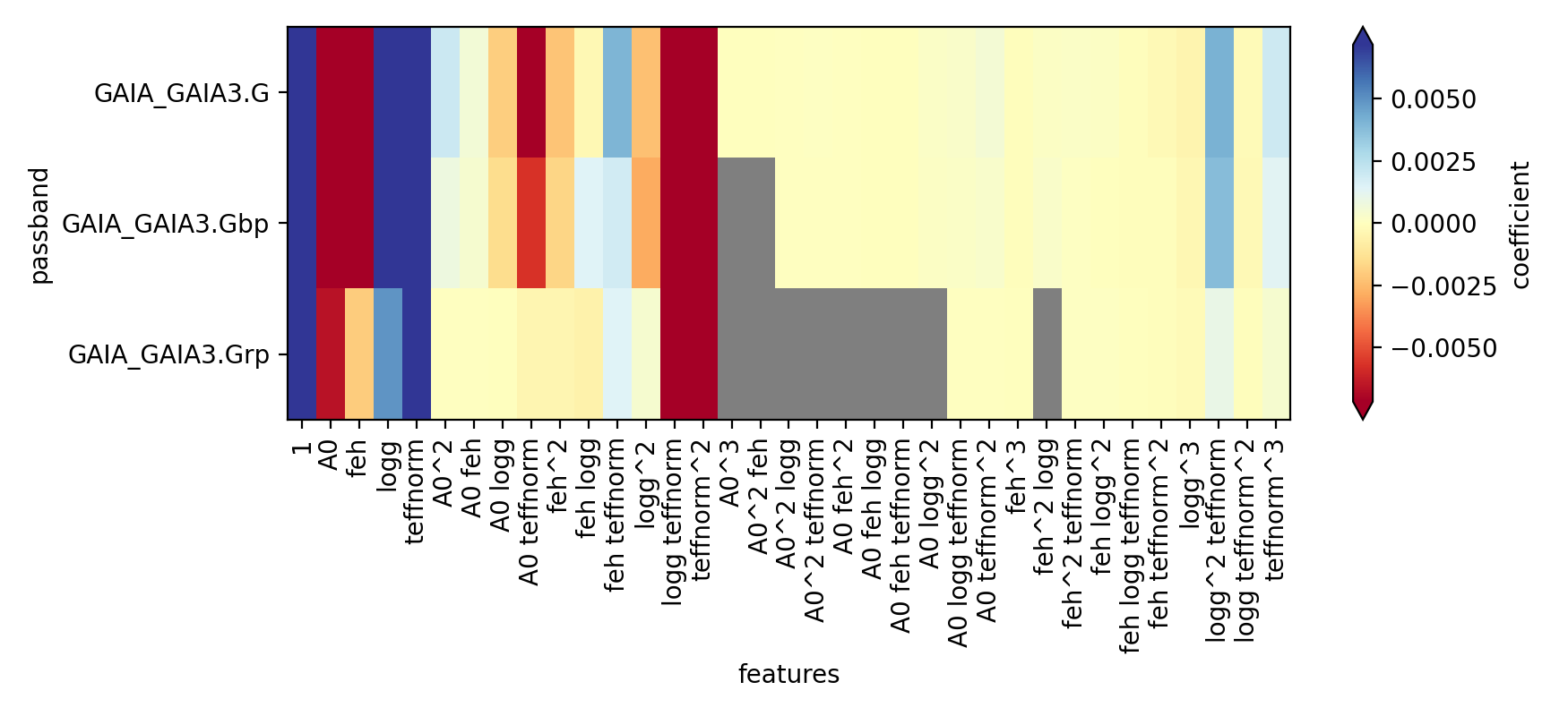
(png, hires.png, pdf) Statistics on polynomial approximation of extinction effect per passband. The top panel shows the residual statistics of the model to the grid values, while the bottom panel shows the meaningful coefficient amplitudes. (Grey pixels indicate values below \(10^{-5}\)).

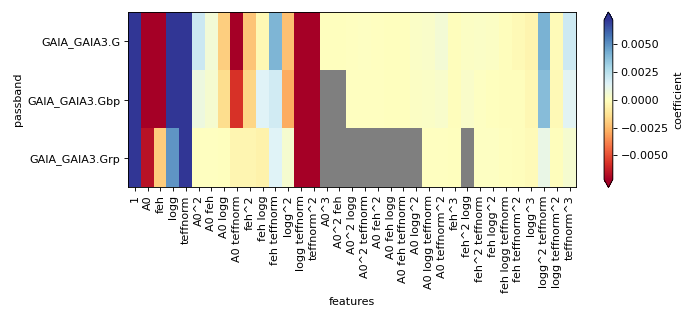
(png, hires.png, pdf) Statistics on polynomial approximation of extinction effect per passband. The top panel shows the residual statistics of the model to the grid values, while the bottom panel shows the meaningful coefficient amplitudes. (Grey pixels indicate values below \(10^{-5}\)).

class dustapprox.models.polynomial.PolynomialModel(**kwargs)

Bases: dustapprox.models.basemodel._BaseModel

A polynomial model object

meta

meta information about the model

Type

dict

transformer_

polynomial transformer

Type

PolynomialFeatures

coeffs_

coefficients of the regression on the polynomial expended features

Type

pd.Series

property degree_: int

Degree of the polynomial transformation

property feature_names: Sequence[str]

Input feature dimensions of the model

fit(df: pandas.core.frame.DataFrame, features: Optional[Sequence[str]] = None, label: str = 'Ax', degree: int = 3, interaction_only: bool = False)

Parameters

• df (DataFrame) – DataFrame with the passband grid data.

• features (Sequence[str]) – input features from df (note: if used, teff will be normalized to teff/5040)

• label (str) – which field contains the label values

• degree (int) – The degree of the polynomial model.

• interaction_only (bool) – If True, only the interaction terms are used.

• input_parameters (Sequence[str]) – The input parameters to use. If None, ‘teff logg feh A0 alpha’ parameters are used.

classmethod from_file(filename: str, passband: str)

Restore a model from a file

Parameters

• filename (str) –

  the ECSV filepath containing the model definition

  The file should contain the various parameters associated with the model in its metadata.

• passband (str) – name of the model to load (passband column in the ecsv file)

Returns

model – model object

Return type

PolynomialModel

get_transformed_feature_names() → Sequence[str]

get the feature names of the internal transformation

property name: str

Get the model name also stored in the coeffs series

predict(X: Union[numpy.ndarray, pandas.core.frame.DataFrame]) → numpy.array

Predict the extinction in the specific passband

Note

if X is a Dataframe, teffnorm could be automatically added

Parameters

X (Union[np.ndarray, pd.DataFrame]) – input features

Returns

y – predicted values

Return type

np.ndarray

to_ecsv(fname: str, **meta)

Export model into an ECSV file

to_pandas() → pandas.core.frame.DataFrame

Export the model to a pandas array, useful for storage

dustapprox.models.polynomial.approx_model(r: pandas.core.frame.DataFrame, passband: str = 'GAIA_GAIA3.G', degree: int = 3, interaction_only: bool = False, input_parameters: Optional[Sequence[str]] = None, verbose=False) → dict

Fit the passband grid data with a polynomial model.

Parameters

• r (DataFrame) – DataFrame with the passband grid data.

• passband (str) – The passband to fit.

• degree (int) – The degree of the polynomial model.

• interaction_only (bool) – If True, only the interaction terms are used.

• input_parameters (Sequence[str]) – The input parameters to use. If None, ‘teff logg feh A0 alpha’ parameters are used.

• verbose (bool) – If True, print the model parameters and statistics

Returns

Dictionary with the model parameters and statistics.

Return type

dict

dustapprox.models.polynomial.quick_plot_models(r: pandas.core.frame.DataFrame, **kwargs) → pandas.core.frame.DataFrame

Plot diagnostic plots for the models.

Parameters

r (DataFrame) – DataFrame with the passband grid data.

Returns

• DataFrame – DataFrame with the all model parameters and statistics.

• .. seealso:: – approx_model()