Introduction to Scikit-learn#
Last update June, 13 2023
%matplotlib inline
import pandas as pd
import numpy as np
import pylab as plt
from IPython.display import Markdown, display
Predicting galaxy redshift via regression on 3D-HST photometry#
Download data#
First, download the 3D-HST catalog from the MAST archive. This dataset is described in Skelton et. al 2014.
from astropy.utils.data import download_file
import tarfile

file_url = 'https://archive.stsci.edu/missions/hlsp/3d-hst/RELEASE_V4.0/Photometry/3dhst_master.phot.v4.1.tar'
tarfile.open(download_file(file_url, cache=True), "r:")\
       .extract('3dhst_master.phot.v4.1/3dhst_master.phot.v4.1.cat', '.')
Read the combined photmetric catalog into a dataframe via astropy
from astropy.table import Table

df = Table.read('3dhst_master.phot.v4.1/3dhst_master.phot.v4.1.cat', format='ascii').to_pandas()
df
| id | field | ra | dec | x | y | z_spec | z_peak | faper_F140W | eaper_F140W | ... | flags | f140w_flag | star_flag | use_phot | near_star | nexp_f125w | nexp_f140w | nexp_f160w | lmass | Av | |
|---|---|---|---|---|---|---|---|---|---|---|---|---|---|---|---|---|---|---|---|---|---|
| 0 | 1.0 | AEGIS | 215.222382 | 53.004185 | 9590.50 | 3057.30 | -1.0000 | 0.0100 | -82.0410 | -82.041000 | ... | 0 | 0 | 1 | 0 | 0 | 2 | 0 | 3 | 7.51 | 1.1 |
| 1 | 2.0 | AEGIS | 215.096588 | 52.918053 | 16473.20 | 3150.20 | -1.0000 | 0.0100 | 3.5078 | 0.074233 | ... | 3 | 0 | 0 | 0 | 0 | 4 | 4 | 4 | 5.62 | 0.1 |
| 2 | 3.0 | AEGIS | 215.161469 | 52.959461 | 13060.10 | 2982.30 | -1.0000 | 0.2062 | -1.9043 | -1.904300 | ... | 1 | 0 | 0 | 1 | 0 | 2 | 0 | 2 | 9.00 | 1.1 |
| 3 | 4.0 | AEGIS | 215.305298 | 53.052921 | 5422.80 | 2692.10 | -1.0000 | 0.0355 | -72.3250 | -72.325000 | ... | 0 | 0 | 0 | 0 | 0 | 1 | 0 | 1 | 4.78 | 0.4 |
| 4 | 5.0 | AEGIS | 215.041840 | 52.871273 | 19894.60 | 2834.40 | -1.0000 | 0.3427 | 1890.5000 | 0.133300 | ... | 0 | 1 | 2 | 0 | 1 | 0 | 3 | 0 | 11.57 | 0.5 |
| ... | ... | ... | ... | ... | ... | ... | ... | ... | ... | ... | ... | ... | ... | ... | ... | ... | ... | ... | ... | ... | ... |
| 207962 | 44098.0 | UDS | 34.363106 | -5.122067 | 14578.84 | 11076.42 | -1.0000 | 0.1852 | 188.8200 | 0.170750 | ... | 0 | 1 | 2 | 0 | 0 | 0 | 3 | 0 | 10.21 | 0.2 |
| 207963 | 44099.0 | UDS | 34.333569 | -5.123219 | 16343.92 | 11007.12 | -1.0000 | 0.6716 | 1.7193 | 0.129080 | ... | 0 | 1 | 2 | 0 | 0 | 0 | 3 | 0 | 8.49 | 0.7 |
| 207964 | 44100.0 | UDS | 34.363682 | -5.123123 | 14544.39 | 11013.01 | 1.4196 | 2.7489 | 1.3829 | 0.113830 | ... | 0 | 1 | 2 | 0 | 0 | 0 | 4 | 0 | 9.08 | 1.4 |
| 207965 | 44101.0 | UDS | 34.556389 | -5.123040 | 3028.23 | 11017.04 | -1.0000 | 1.1716 | -99.0000 | -99.000000 | ... | 1 | 0 | 0 | 0 | 0 | 1 | 0 | 2 | 10.55 | 1.0 |
| 207966 | 44102.0 | UDS | 34.365097 | -5.121975 | 14459.90 | 11081.91 | -1.0000 | 0.6160 | 1.5335 | 0.152730 | ... | 0 | 1 | 2 | 0 | 0 | 0 | 3 | 0 | 8.58 | 0.0 |
207967 rows × 38 columns
Exploring the dataset#
Now we will examine the contents of the catalog.
The dataset contains standard information such as target id, field name, coordinates (ra, dec), fluxes, uncertainties, and various photometric flags (see Skelton et. al 2014, or download the README here).
In addition, there are some derived properties such as photometric redshift (z_peak), spectroscopic redshift (z_spec), mass (lmass) and dust extinction in the V band (Av).
Kriek et al (2018; FAST) describe the masse estimates.
Keep in mind that we are interested in predicting redshift, so our “target” variable will be z_spec. The “features” will be all relevant columns.
# Your turn to explore for ~5 minutes.
df.columns
Index(['id', 'field', 'ra', 'dec', 'x', 'y', 'z_spec', 'z_peak', 'faper_F140W',
       'eaper_F140W', 'faper_F160W', 'eaper_F160W', 'f_F606W', 'e_F606W',
       'f_F814W', 'e_F814W', 'f_F125W', 'e_F125W', 'f_F140W', 'e_F140W',
       'f_F160W', 'e_F160W', 'tot_cor', 'kron_radius', 'a_image', 'b_image',
       'flux_radius', 'fwhm_image', 'flags', 'f140w_flag', 'star_flag',
       'use_phot', 'near_star', 'nexp_f125w', 'nexp_f140w', 'nexp_f160w',
       'lmass', 'Av'],
      dtype='object')
df.describe().T
| count | mean | std | min | 25% | 50% | 75% | max | |
|---|---|---|---|---|---|---|---|---|
| id | 207967.0 | 2.117321e+04 | 1.265041e+04 | 1.000000 | 10399.000000 | 20797.000000 | 31195.500000 | 5.050700e+04 |
| ra | 207967.0 | 1.220675e+02 | 7.383123e+01 | 34.216633 | 53.061646 | 150.091034 | 189.306900 | 2.153053e+02 |
| dec | 207967.0 | 1.446509e+01 | 3.538768e+01 | -27.959742 | -5.272032 | 2.274822 | 52.957975 | 6.238830e+01 |
| x | 207967.0 | 1.215648e+04 | 7.233914e+03 | 7.400000 | 7316.685000 | 10578.100000 | 15137.135000 | 3.766890e+04 |
| y | 207967.0 | 1.023374e+04 | 5.733813e+03 | 1273.020000 | 6161.300000 | 8873.450000 | 13184.660000 | 3.075330e+04 |
| z_spec | 207967.0 | -9.536530e-01 | 4.891243e-01 | -99.900000 | -1.000000 | -1.000000 | -1.000000 | 6.118000e+00 |
| z_peak | 207967.0 | 1.177393e+00 | 6.727479e+00 | -99.000000 | 0.817400 | 1.415900 | 2.128050 | 5.960900e+00 |
| faper_F140W | 207967.0 | -1.542424e+01 | 3.237767e+02 | -482.630000 | -48.633500 | 0.178810 | 0.491190 | 4.705200e+04 |
| eaper_F140W | 207967.0 | -2.211378e+01 | 5.445781e+01 | -482.630000 | -48.633500 | 0.069309 | 0.086337 | 1.059200e+04 |
| faper_F160W | 207967.0 | 1.339273e+01 | 5.961002e+02 | -99.000000 | 0.186090 | 0.355380 | 0.939190 | 9.118500e+04 |
| eaper_F160W | 207967.0 | -5.187644e-01 | 7.605170e+00 | -99.000000 | 0.026516 | 0.035040 | 0.042530 | 4.745600e+02 |
| f_F606W | 207967.0 | -7.108241e+00 | 9.912538e+01 | -99.000000 | 0.070850 | 0.188050 | 0.488610 | 1.453600e+04 |
| e_F606W | 207967.0 | 1.313269e+16 | 3.789337e+18 | -99.000000 | 0.020005 | 0.029607 | 0.039982 | 1.503200e+21 |
| f_F814W | 207967.0 | -2.199676e+01 | 1.390750e+02 | -99.000000 | -99.000000 | 0.176220 | 0.528775 | 1.786700e+04 |
| e_F814W | 207967.0 | 3.236528e+16 | 6.628122e+18 | -99.000000 | -99.000000 | 0.033730 | 0.051859 | 1.804100e+21 |
| f_F125W | 207967.0 | 1.623084e+01 | 6.283784e+02 | -99.000000 | 0.227010 | 0.487080 | 1.381500 | 1.144900e+05 |
| e_F125W | 207967.0 | -4.258125e-01 | 1.319884e+01 | -99.000000 | 0.053360 | 0.070784 | 0.095966 | 2.480300e+03 |
| f_F140W | 207967.0 | -1.702118e+01 | 4.170184e+02 | -99.000000 | -99.000000 | 0.257440 | 0.822930 | 6.653000e+04 |
| e_F140W | 207967.0 | -2.656068e+01 | 8.092820e+01 | -99.000000 | -99.000000 | 0.101650 | 0.141770 | 2.068100e+04 |
| f_F160W | 207967.0 | 1.956213e+01 | 8.029663e+02 | -99.000000 | 0.265040 | 0.568550 | 1.652050 | 1.308100e+05 |
| e_F160W | 207967.0 | -3.964592e-01 | 1.964629e+01 | -99.000000 | 0.051773 | 0.075900 | 0.114420 | 8.075000e+03 |
| tot_cor | 207967.0 | 1.115344e+00 | 5.067883e-02 | 1.000000 | 1.076500 | 1.118200 | 1.151900 | 1.210700e+00 |
| kron_radius | 207967.0 | 4.649582e+00 | 4.175856e+00 | -99.000000 | 3.580000 | 4.460000 | 5.650000 | 1.017000e+01 |
| a_image | 207967.0 | 3.071895e+00 | 4.629618e+00 | -99.000000 | 1.840000 | 2.530000 | 3.740000 | 1.540020e+02 |
| b_image | 207967.0 | 2.115423e+00 | 4.147367e+00 | -99.000000 | 1.396000 | 1.913000 | 2.604500 | 7.131000e+01 |
| flux_radius | 207967.0 | 4.191743e+00 | 3.429291e+01 | -5480.000000 | 2.930000 | 3.720000 | 5.000000 | 1.340000e+04 |
| fwhm_image | 207967.0 | 1.996158e-01 | 4.746242e+00 | -99.000000 | 0.000000 | 0.000000 | 0.000000 | 5.367900e+02 |
| flags | 207967.0 | 5.006419e-01 | 1.278831e+00 | 0.000000 | 0.000000 | 0.000000 | 0.000000 | 2.300000e+01 |
| f140w_flag | 207967.0 | 3.303409e-03 | 5.738042e-02 | 0.000000 | 0.000000 | 0.000000 | 0.000000 | 1.000000e+00 |
| star_flag | 207967.0 | 1.310165e+00 | 9.436616e-01 | 0.000000 | 0.000000 | 2.000000 | 2.000000 | 2.000000e+00 |
| use_phot | 207967.0 | 8.470046e-01 | 3.599840e-01 | 0.000000 | 1.000000 | 1.000000 | 1.000000 | 1.000000e+00 |
| near_star | 207967.0 | 4.426664e-02 | 2.056874e-01 | 0.000000 | 0.000000 | 0.000000 | 0.000000 | 1.000000e+00 |
| nexp_f125w | 207967.0 | 8.358509e+00 | 1.091935e+01 | 0.000000 | 4.000000 | 4.000000 | 8.000000 | 9.100000e+01 |
| nexp_f140w | 207967.0 | 4.425048e+00 | 9.310295e+00 | 0.000000 | 0.000000 | 4.000000 | 4.000000 | 8.400000e+01 |
| nexp_f160w | 207967.0 | 9.051638e+00 | 1.519260e+01 | 0.000000 | 4.000000 | 4.000000 | 8.000000 | 1.320000e+02 |
| lmass | 207967.0 | 8.410625e+00 | 1.511090e+00 | -1.000000 | 7.910000 | 8.500000 | 9.180000 | 1.463000e+01 |
| Av | 207967.0 | 3.189294e-01 | 5.449457e-01 | -1.000000 | 0.000000 | 0.100000 | 0.500000 | 4.000000e+00 |
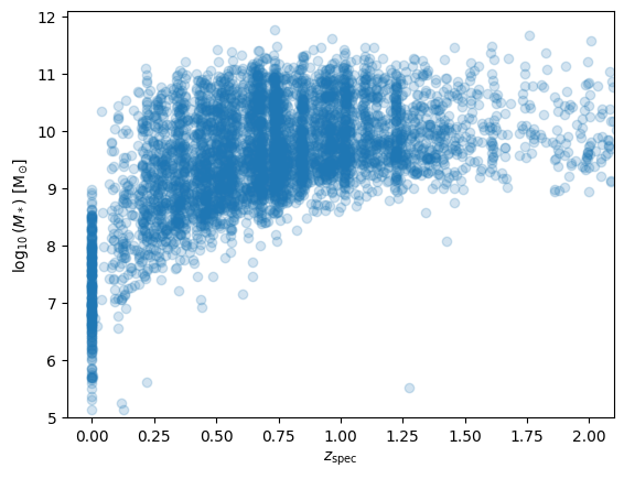
ax = plt.subplot(111)

ax.scatter(df.z_spec, df.lmass, alpha=0.2)
ax.set_xlabel(r'$z_{\rm spec}$')
ax.set_ylabel(r'$\log_{10}{(M_*)}$ [M$_{\odot}$]')
ax.set_xlim(-0.1, 2.1)
ax.set_ylim(5., 12.1);
display(Markdown("""
> Physical parameters mass vs. redshift.
We find a pileup of redshit estimates at 0 and even negative estimates. In addition, some
masses are negative. These need to be cleaned for further uses.
"""))
Physical parameters mass vs. redshift. We find a pileup of redshit estimates at 0 and even negative estimates. In addition, some masses are negative. These need to be cleaned for further uses.
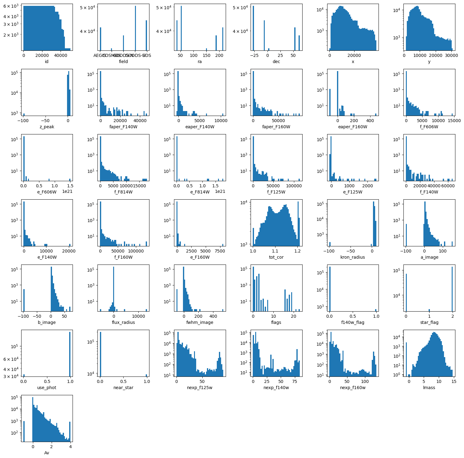
columns = [k for k in df.columns if k != 'z_spec']

wrap = 6

plt.figure(figsize=(15, 15))

nlines = len(columns) // wrap +  int(len(columns) % wrap > 0)

for e, colname in enumerate(columns, 1):
    plt.subplot(nlines, wrap, e)
    plt.hist(df[colname], bins=43, log=True)
    plt.xlabel(colname)

plt.tight_layout()
Perform data cleaning & select features#
Before building and applying a regression model, we first need to inspect and clean the dataset.
Cleaning:
only keep sources with \(log(M)>9\) to remove sources which do not have complete coverage across redshift.
remove redshift = 0
We do not keep
z_photto avoid leakage.The
Av,lmassandz_peakvalues come from the FAST photometric fit, and so we will exclude them as well.We will exclude the categorical flag variables (‘flags’, ‘f140w_flag’, ‘star_flag’, ‘use_phot’, ‘near_star’).
remove = ('Av', 'lmass', 'z_peak', 'flags', 'f140w_flag', 'star_flag',
          'use_phot', 'near_star', 'z_spec', 'id', 'field',
          'ra', 'dec', 'x', 'y')
features = [col for col in df.columns if col not in remove]

target = 'z_spec'

Markdown(f"""
**features** {features}

**target**: {target} """)
features [‘faper_F140W’, ‘eaper_F140W’, ‘faper_F160W’, ‘eaper_F160W’, ‘f_F606W’, ‘e_F606W’, ‘f_F814W’, ‘e_F814W’, ‘f_F125W’, ‘e_F125W’, ‘f_F140W’, ‘e_F140W’, ‘f_F160W’, ‘e_F160W’, ‘tot_cor’, ‘kron_radius’, ‘a_image’, ‘b_image’, ‘flux_radius’, ‘fwhm_image’, ‘nexp_f125w’, ‘nexp_f140w’, ‘nexp_f160w’]
target: z_spec
Filter data and impute missing values#
We need to transform text into values/categories.
from sklearn.preprocessing import LabelEncoder
df['field_lbl'] = LabelEncoder().fit_transform(df['field'])
By inspection of mass vs redshift, we will only keep sources with \(log(M)>9\) to remove sources that do not have complete coverage across redshift.
df = df[(df[target] > 0) & (df['lmass'] > 9)]
We use the median of the distributions to replace bad / missing values
ecols = [col for col in features if (col[0] == 'e') and (col[-1] == 'W')]

for col in ecols:
    missing_value = np.nanmedian(df[col])
    df.loc[df[col] < -90, col] = missing_value
df_x = df[features]
df_y = df[target]
df_x
| faper_F140W | eaper_F140W | faper_F160W | eaper_F160W | f_F606W | e_F606W | f_F814W | e_F814W | f_F125W | e_F125W | ... | e_F160W | tot_cor | kron_radius | a_image | b_image | flux_radius | fwhm_image | nexp_f125w | nexp_f140w | nexp_f160w | |
|---|---|---|---|---|---|---|---|---|---|---|---|---|---|---|---|---|---|---|---|---|---|
| 26 | -71.0650 | -71.065000 | 8.1873 | 0.049477 | 3.8503 | 0.036320 | 6.3439 | 0.055958 | 9.9996 | 0.079702 | ... | 0.11941 | 1.0931 | 3.50 | 3.730 | 3.210 | 3.38 | 0.00 | 2 | 0 | 2 |
| 69 | -60.6090 | -60.609000 | 3.2127 | 0.052521 | 1.5757 | 0.041291 | 2.6588 | 0.062491 | 4.8744 | 0.093860 | ... | 0.16605 | 1.0717 | 4.37 | 3.750 | 3.140 | 4.28 | 0.00 | 2 | 0 | 2 |
| 82 | -40.9920 | -40.992000 | 6.4949 | 0.052284 | 4.4121 | 0.059577 | 8.6526 | 0.092122 | 14.5010 | 0.135510 | ... | 0.23213 | 1.0456 | 3.62 | 5.560 | 5.260 | 6.59 | 0.00 | 2 | 0 | 2 |
| 144 | -33.7210 | -33.721000 | 2.2822 | 0.035636 | 2.3501 | 0.075882 | 4.2912 | 0.118310 | 6.0816 | 0.115550 | ... | 0.16608 | 1.0420 | 3.50 | 7.370 | 4.590 | 7.78 | 0.00 | 4 | 0 | 4 |
| 154 | -54.5630 | -54.563000 | 4.6583 | 0.055052 | 1.8658 | 0.044419 | 3.4657 | 0.067187 | 6.3630 | 0.104380 | ... | 0.20044 | 1.0623 | 4.08 | 5.500 | 3.070 | 5.04 | 0.00 | 2 | 0 | 2 |
| ... | ... | ... | ... | ... | ... | ... | ... | ... | ... | ... | ... | ... | ... | ... | ... | ... | ... | ... | ... | ... | ... |
| 205837 | -99.0000 | 0.065174 | 30.6860 | 0.032872 | 6.2959 | 0.062144 | 19.7480 | 0.062613 | 51.5940 | 0.159870 | ... | 0.22079 | 1.0280 | 3.50 | 9.057 | 5.362 | 7.00 | 10.32 | 4 | 0 | 4 |
| 206257 | -99.0000 | 0.065174 | 58.5290 | 0.033204 | 15.0210 | 0.075732 | 45.7970 | 0.075405 | 129.2900 | 0.198170 | ... | 0.50738 | 1.0000 | 3.50 | 13.952 | 12.710 | 9.53 | 7.50 | 4 | 0 | 4 |
| 207042 | -99.0000 | 0.065174 | 41.6890 | 0.048789 | 102.7100 | 0.306440 | 158.0200 | 0.351600 | 298.0700 | 0.533640 | ... | 0.74396 | 1.0000 | 3.50 | 21.379 | 8.268 | 16.90 | 43.85 | 4 | 0 | 4 |
| 207646 | -99.0000 | 0.065174 | 13.4370 | 0.054057 | 7.3063 | 0.044850 | 9.1046 | 0.045867 | 11.2820 | 0.147020 | ... | 0.14652 | 1.0985 | 3.50 | 3.522 | 3.125 | 2.84 | 4.52 | 2 | 0 | 2 |
| 207964 | 1.3829 | 0.113830 | -99.0000 | 0.033797 | 1.1099 | 0.065573 | 1.3620 | 0.065967 | -99.0000 | 0.092815 | ... | 0.18208 | 1.0743 | 5.90 | 3.040 | 1.942 | 5.25 | 0.00 | 0 | 4 | 0 |
4173 rows × 23 columns
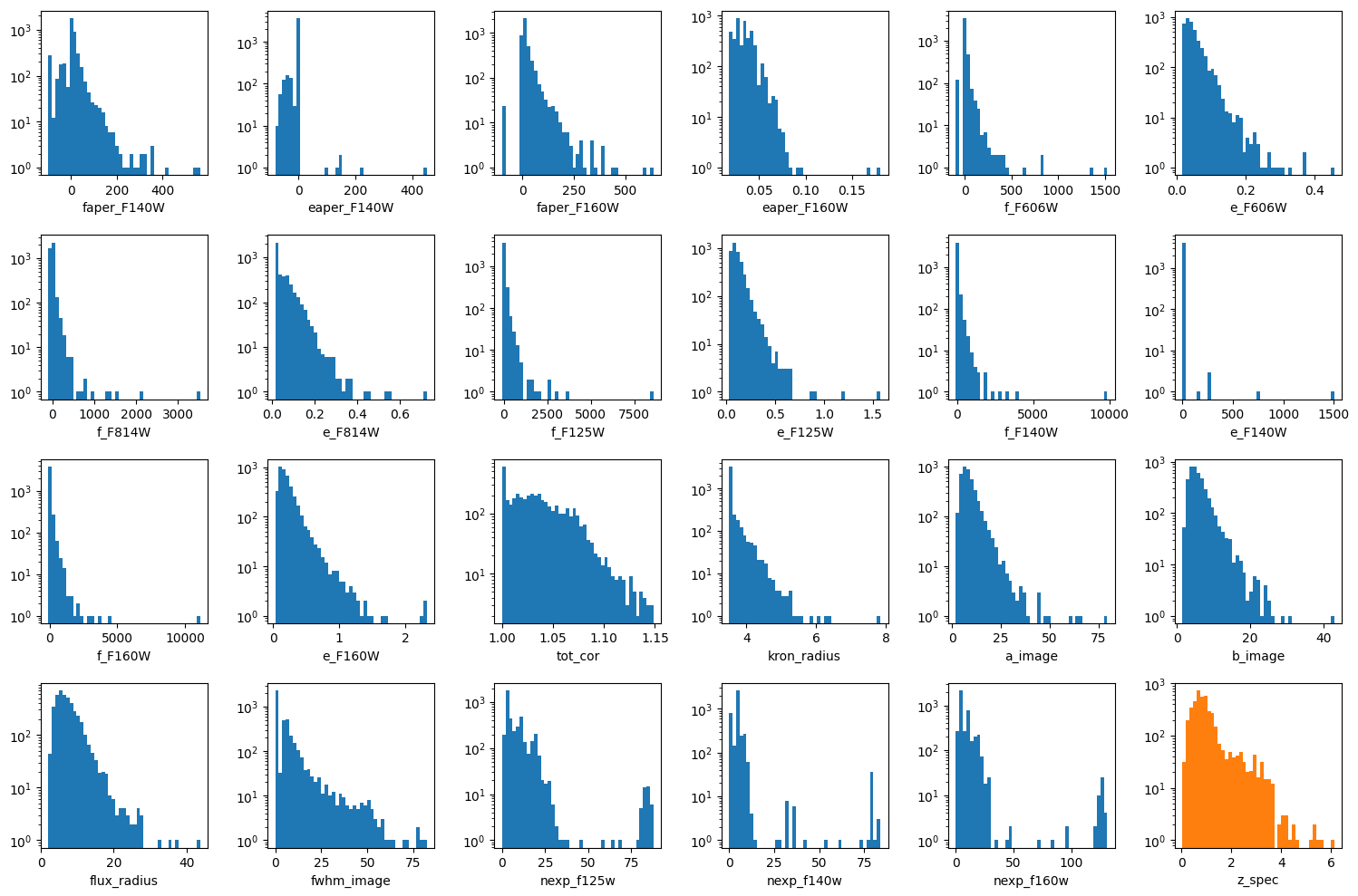
columns = [k for k in df_x.columns]

wrap = 6

plt.figure(figsize=(15, 10))

nlines = (len(columns) + 1) // wrap +  int((len(columns) + 1) % wrap > 0)

for e, colname in enumerate(columns, 1):
    plt.subplot(nlines, wrap, e)
    plt.hist(df_x[colname], bins=43, log=True)
    plt.xlabel(colname)

plt.subplot(nlines, wrap, e + 1)
plt.hist(df_y, bins=43, log=True, color='C1')
plt.xlabel(target)

plt.tight_layout()
Divide the data into train, test and validation sets#
Note that typically one needs to pass arrays to the common libraries.
X = df[features].values
y = df[target].values
However, Scikit-learn has implemented pandas interfaces, so we do not need to do so in this particular exercise.
Divide the data into train, validation and test sets. We will use the following definitions:
Training: The data used to update model parameters (e.g., coefficients or matrix element values).
Validation: The data used to update model selection (for instance, we might change hyperparameters of a model based on the validation metrics).
Testing: The data used to make final predictions, and possibly evaluate the final model score.
from sklearn.model_selection import train_test_split

# first reserve 70% of the data for training, 30% for validation
X_train, X_test, y_train, y_test = train_test_split(df_x, df_y, test_size=0.1, random_state=42)

# second, split the validation set in half to obtain validation and test sets.
#X_validate, X_test, y_validate, y_test = train_test_split(X_validate, y_validate, test_size=0.5, random_state=42)
Explore regression models#
Here we explore a few options for regressor models.
Linear Regression#
Let’s do a simple one first
from sklearn.linear_model import LinearRegression
lin = LinearRegression()
lin.fit(X_train, y_train)
LinearRegression()In a Jupyter environment, please rerun this cell to show the HTML representation or trust the notebook.
On GitHub, the HTML representation is unable to render, please try loading this page with nbviewer.org.
LinearRegression()
lin.coef_, lin.intercept_
(array([-1.12407403e-03,  4.98219553e-03, -6.70675227e-04, -1.06634270e+01,
         1.11381308e-04, -1.39065803e+00, -2.61477442e-04, -8.17271081e-02,
        -4.42902735e-03,  2.80098384e-01,  5.33909891e-05, -1.13781321e-03,
         3.46999047e-03,  3.68519285e-01,  1.35567665e+01,  6.38453228e-01,
        -1.47687629e-02,  2.22513476e-02,  1.72805797e-02, -6.25811132e-03,
         1.74102852e-02,  4.26894552e-03, -1.31612712e-02]),
 -15.146015762740168)
To quantify the performance of the model, we will apply it to the validation set and compare the predicted values with the true values by computing the mean squared error:
from sklearn.metrics import mean_squared_error

y_predict = lin.predict(X_test)
y_predict0 = lin.predict(X_train)
mse = mean_squared_error(y_test, y_predict)
print(f'MSE = {mse:.4f}')

fig, ax = plt.subplots(1, 1, figsize=(4, 4))
ax.scatter(y_test, y_predict, alpha=0.2, label='test')
ax.scatter(y_train, y_predict0, alpha=0.2, label='train', zorder=-1)
ax.plot(ax.get_xlim(), ax.get_xlim(), zorder=-1, color='0.5')
ax.set_aspect('equal')
ax.set_xlim(-0.1, 5)
ax.set_ylim(-0.1, 5)
ax.grid()
ax.set_xlabel('Truth (y_test)')
ax.set_ylabel('Prediction (y_predict)')
plt.legend(loc='upper left')
ax.text(0.9, 0.9, f"MSE={mse:0.4f}", transform=ax.transAxes, ha='right');
MSE = 0.3198
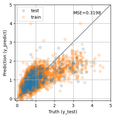
The MSE is not great. Not surprising given the simplicity of our model. Maybe we can do better changing the model?
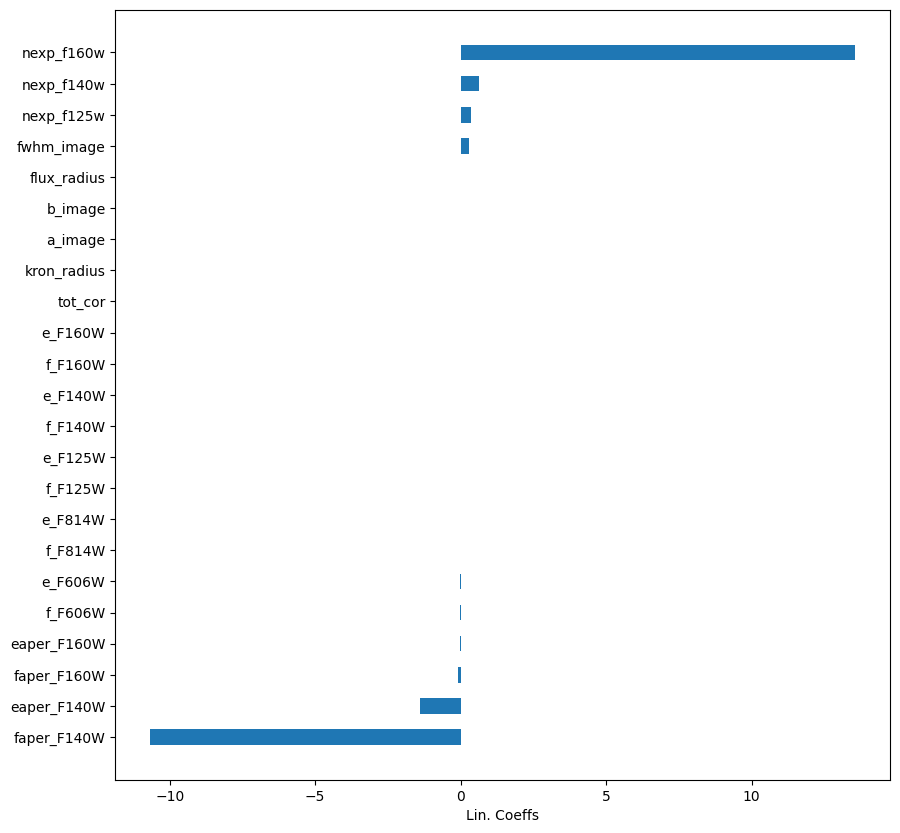
importances = lin.coef_
labels = lin.feature_names_in_
argsort = np.argsort(importances)
fig = plt.figure(figsize=[10, 10])
ax = fig.add_subplot(111)
ax.barh(np.arange(len(df_x.columns)), importances[argsort],
        align='center',
        height=0.5,
        tick_label=labels)
ax.set_xlabel("Lin. Coeffs")
Text(0.5, 0, 'Lin. Coeffs')
from sklearn.pipeline import Pipeline
from sklearn.preprocessing import PolynomialFeatures, StandardScaler
from sklearn.linear_model import LassoLarsIC

pipe = Pipeline([
    ('polynomial', PolynomialFeatures(degree=3)),
    ('scaler', StandardScaler()),
    ('classifier', LassoLarsIC(normalize=False))
])

pipe.fit(X_train, y_train)
---------------------------------------------------------------------------
TypeError                                 Traceback (most recent call last)
Cell In[22], line 8
      2 from sklearn.preprocessing import PolynomialFeatures, StandardScaler
      3 from sklearn.linear_model import LassoLarsIC
      5 pipe = Pipeline([
      6     ('polynomial', PolynomialFeatures(degree=3)),
      7     ('scaler', StandardScaler()),
----> 8     ('classifier', LassoLarsIC(normalize=False))
      9 ])
     11 pipe.fit(X_train, y_train)

TypeError: __init__() got an unexpected keyword argument 'normalize'
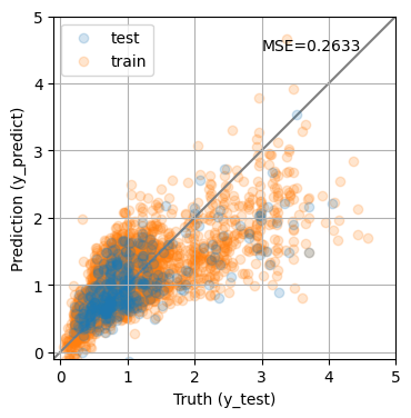
y_predict = pipe.predict(X_test)
y_predict0 = pipe.predict(X_train)
mse = mean_squared_error(y_test, y_predict)
print(f'MSE = {mse:.4f}')

fig, ax = plt.subplots(1, 1, figsize=(4, 4))
ax.scatter(y_test, y_predict, alpha=0.2, label='test')
ax.scatter(y_train, y_predict0, alpha=0.2, label='train', zorder=-1)
ax.plot(ax.get_xlim(), ax.get_xlim(), zorder=-1, color='0.5')
ax.set_aspect('equal')
ax.set_xlim(-0.1, 5)
ax.set_ylim(-0.1, 5)
ax.grid()
ax.set_xlabel('Truth (y_test)')
ax.set_ylabel('Prediction (y_predict)')
plt.legend(loc='best')
ax.text(0.9, 0.9, f"MSE={mse:0.4f}", transform=ax.transAxes, ha='right');
MSE = 0.2633
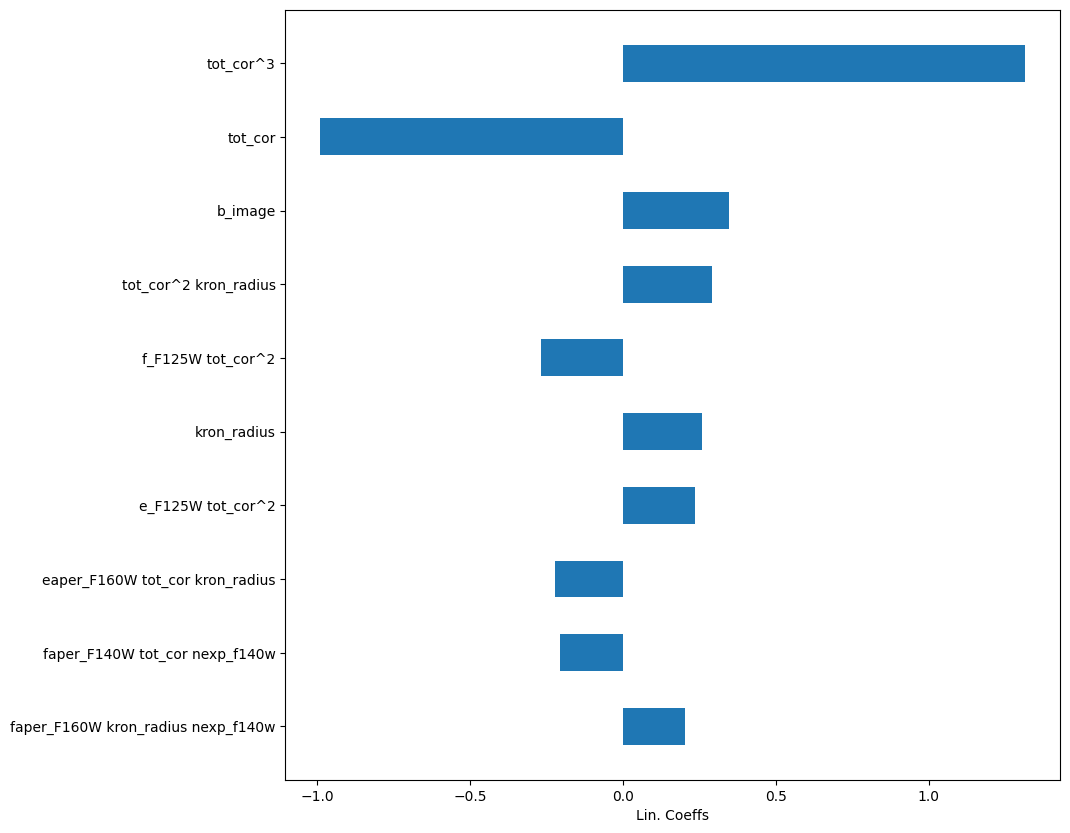
importances = pipe['classifier'].coef_
labels = pipe['polynomial'].get_feature_names_out()
argsort = np.argsort(np.abs(importances))[-10:]

importances = importances[argsort]
labels = labels[argsort]

fig = plt.figure(figsize=[10, 10])
ax = fig.add_subplot(111)
ax.barh(np.arange(len(labels)), importances,
        align='center',
        height=0.5,
        tick_label=labels)
ax.set_xlabel("Lin. Coeffs")
Text(0.5, 0, 'Lin. Coeffs')
Other models#
Using sklearn, it is very easy to change a model for something different.
Random Forest#
Using sklearn, we can very easily construct a decision tree model for regressing redshift from the photometric catalog features. A decision tree is composed of a series of if-else decision steps. The number of steps and the types of decision at each step is determined by training the algorithm with supervision. In this first example, we will use the DecisionTreeRegressor from sklearn.
from sklearn.ensemble import RandomForestRegressor

# use the same parameters as the Decision Tree
params = {
    "min_samples_split": 15,
    "min_samples_leaf": 5,
    "max_depth": 15,
}

# Initialize the model
rf = RandomForestRegressor(**params)

rf.fit(X_train, y_train)
RandomForestRegressor(max_depth=15, min_samples_leaf=5, min_samples_split=15)In a Jupyter environment, please rerun this cell to show the HTML representation or trust the notebook.
On GitHub, the HTML representation is unable to render, please try loading this page with nbviewer.org.
RandomForestRegressor(max_depth=15, min_samples_leaf=5, min_samples_split=15)
y_predict = rf.predict(X_test)
y_predict0 = rf.predict(X_train)
mse = mean_squared_error(y_test, y_predict)
print(f'MSE = {mse:.4f}')

fig, ax = plt.subplots(1, 1, figsize=(4, 4))
ax.scatter(y_test, y_predict, alpha=0.2, label='test')
ax.scatter(y_train, y_predict0, alpha=0.2, label='train', zorder=-1)
ax.plot(ax.get_xlim(), ax.get_xlim(), zorder=-1, color='0.5')
ax.set_aspect('equal')
ax.set_xlim(-0.1, 5)
ax.set_ylim(-0.1, 5)
ax.set_xlabel('Truth (y_test)')
ax.set_ylabel('Prediction (y_predict)')
plt.legend(loc='best')
ax.text(0.9, 0.9, f"MSE={mse:0.4f}", transform=ax.transAxes, ha='right');
MSE = 0.1182
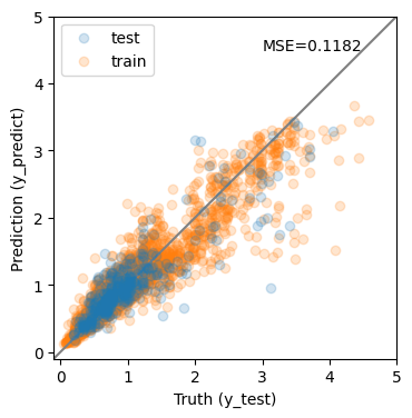
The results are much improved by the random forest!
However, we must be cautious. It is possible that this model suffers from over-fitting. To visualize overfitting, we can compare the mean squared error (MSE) for models of increasing max_depth on the training and testing sets:
max_depths = np.arange(1, 20, 2).astype(int)

train_mse = []
test_mse = []

params = {
    "min_samples_split": 15,
    "min_samples_leaf": 5,
}

for depth in max_depths:

    rff_ = RandomForestRegressor(max_depth=depth, **params)
    rff_.fit(X_train, y_train)

    y_predict_train = rff_.predict(X_train)
    y_predict_test = rff_.predict(X_test)

    train_mse.append(mean_squared_error(y_train, y_predict_train))
    test_mse.append(mean_squared_error(y_test, y_predict_test))


fig, ax = plt.subplots(1, 1)

ax.plot(max_depths, train_mse, color='blue', label='Training Set')
ax.plot(max_depths, test_mse, color='orange', label='Test Set')
ax.set_xlabel('max depth')
ax.set_ylabel('MSE')
ax.legend()
<matplotlib.legend.Legend at 0x119370dc0>
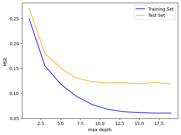
Beyond a max_depth of ~10, the MSE on the training set declines while the MSE on the test set flattens out, suggesting some amount of over-fitting.
To explore further, we will explore how general our model performance (here quantifed with MSE) is using k-fold cross-validation via sklearn. In practice, the X and y datasets are split into k “folds”, and over k iterations, the model is trained using k-1 folds as training data and the remaining fold as a test set to compute performace (i.e., MSE).
from sklearn.model_selection import cross_validate

cv = cross_validate(
    estimator=rf,
    X=df_x,
    y=df_y,
    cv=5, # number of folds
    scoring='neg_mean_squared_error'
)

print(f'Cross-validated score: {cv["test_score"].mean():.3f} +/- {cv["test_score"].std():.3f}')
Cross-validated score: -0.143 +/- 0.056
The previous MSE is consistent with the cross-validated MSE, suggesting that the model is not significantly over-fitting.
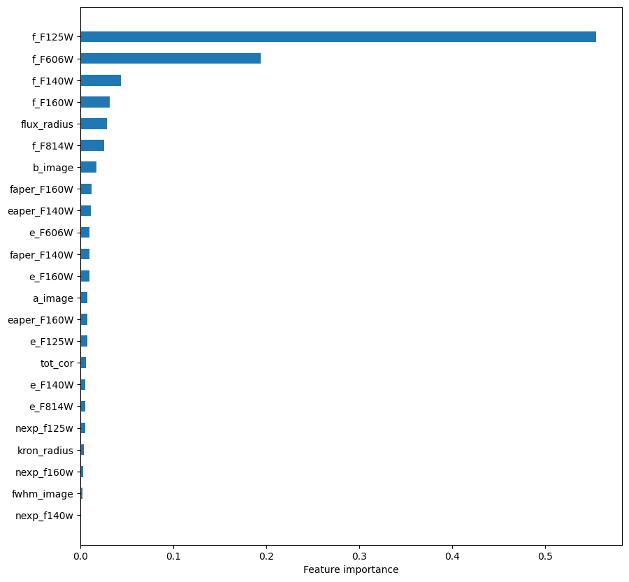
Next, we’ll observe which features are most important to the model predictions.
importances = rf.feature_importances_
argsort = np.argsort(importances)
fig = plt.figure(figsize=[10, 10])
ax = fig.add_subplot(111)
ax.barh(np.arange(len(df_x.columns)), importances[argsort],
        align='center',
        height=0.5,
        tick_label=np.array(features)[argsort])
ax.set_xlabel("Feature importance")
Text(0.5, 0, 'Feature importance')
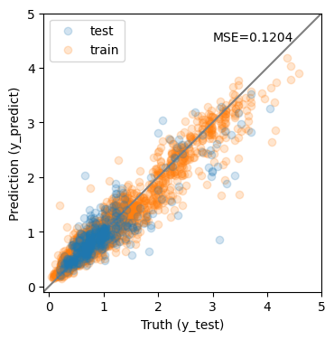
Extratrees#
from sklearn.ensemble import HistGradientBoostingRegressor


# Initialize the model
et = HistGradientBoostingRegressor()

et.fit(X_train, y_train)
HistGradientBoostingRegressor()In a Jupyter environment, please rerun this cell to show the HTML representation or trust the notebook.
On GitHub, the HTML representation is unable to render, please try loading this page with nbviewer.org.
HistGradientBoostingRegressor()
y_predict = et.predict(X_test)
y_predict0 = et.predict(X_train)
mse = mean_squared_error(y_test, y_predict)
print(f'MSE = {mse:.4f}')

fig, ax = plt.subplots(1, 1, figsize=(4, 4))
ax.scatter(y_test, y_predict, alpha=0.2, label='test')
ax.scatter(y_train, y_predict0, alpha=0.2, label='train', zorder=-1)
ax.plot(ax.get_xlim(), ax.get_xlim(), zorder=-1, color='0.5')
ax.set_aspect('equal')
ax.set_xlim(-0.1, 5)
ax.set_ylim(-0.1, 5)
ax.set_xlabel('Truth (y_test)')
ax.set_ylabel('Prediction (y_predict)')
plt.legend(loc='best')
ax.text(0.9, 0.9, f"MSE={mse:0.4f}", transform=ax.transAxes, ha='right');
MSE = 0.1204
cv = cross_validate(
    estimator=et,
    X=df_x,
    y=df_y,
    cv=5, # number of folds
    scoring='neg_mean_squared_error'
)

print(f'Cross-validated score: {cv["test_score"].mean():.3f} +/- {cv["test_score"].std():.3f}')
Cross-validated score: -0.144 +/- 0.053
pipe2 = Pipeline([
    ('polynomial', PolynomialFeatures(degree=3)),
    ('scaler', StandardScaler()),
    ('classifier', HistGradientBoostingRegressor())
])

pipe2.fit(X_train, y_train)
Pipeline(steps=[('polynomial', PolynomialFeatures(degree=3)),
                ('scaler', StandardScaler()),
                ('classifier', HistGradientBoostingRegressor())])
In a Jupyter environment, please rerun this cell to show the HTML representation or trust the notebook. On GitHub, the HTML representation is unable to render, please try loading this page with nbviewer.org.
Pipeline(steps=[('polynomial', PolynomialFeatures(degree=3)),
                ('scaler', StandardScaler()),
('classifier', HistGradientBoostingRegressor())])PolynomialFeatures(degree=3)
StandardScaler()
HistGradientBoostingRegressor()
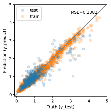
y_predict = pipe2.predict(X_test)
y_predict0 = pipe2.predict(X_train)
mse = mean_squared_error(y_test, y_predict)
print(f'MSE = {mse:.4f}')

fig, ax = plt.subplots(1, 1, figsize=(4, 4))
ax.scatter(y_test, y_predict, alpha=0.2, label='test')
ax.scatter(y_train, y_predict0, alpha=0.2, label='train', zorder=-1)
ax.plot(ax.get_xlim(), ax.get_xlim(), zorder=-1, color='0.5')
ax.set_aspect('equal')
ax.set_xlim(-0.1, 5)
ax.set_ylim(-0.1, 5)
ax.set_xlabel('Truth (y_test)')
ax.set_ylabel('Prediction (y_predict)')
plt.legend(loc='best')
ax.text(0.9, 0.9, f"MSE={mse:0.4f}", transform=ax.transAxes, ha='right');
MSE = 0.1082
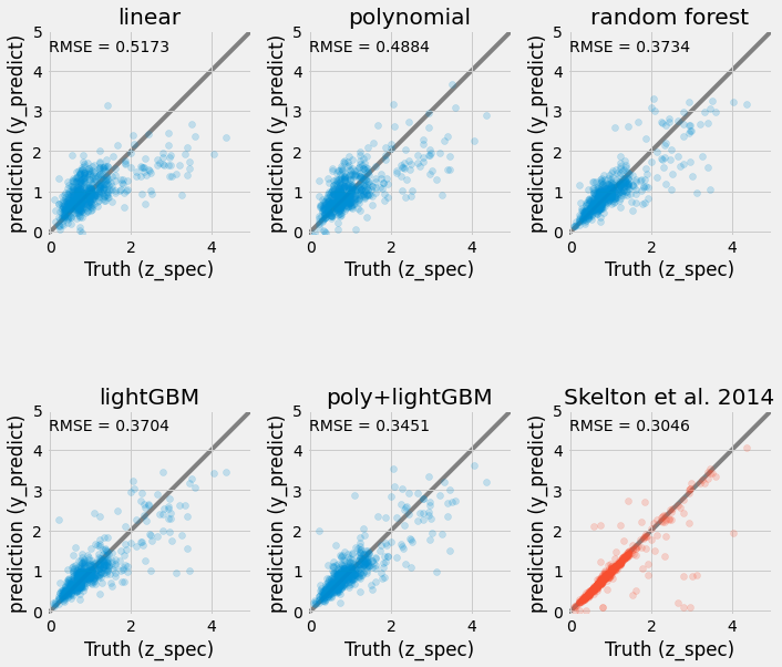
Check against each other and reference#
y_values = [lin.predict(X_test),
            pipe.predict(X_test),
            rf.predict(X_test),
            et.predict(X_test),
            pipe2.predict(X_test),
            df['z_peak'].loc[X_test.index]
]

names = ['linear', 'polynomial', 'random forest', 'lightGBM', 'poly+lightGBM', 'Skelton et al. 2014']


fig, ax = plt.subplots(2, len(names) // 2 , figsize=(10, 10))

for k, (ax, yval) in enumerate(zip(np.ravel(ax), y_values)):
    color = 'C0'
    if k == len(names) - 1:
        color = 'C1'
    ax.scatter(y_test, yval, alpha=0.2, color=color)
    ax.set_aspect('equal')
    ax.set_xlim(-0.1, 5)
    ax.set_ylim(-0.1, 5)
    ax.plot(ax.get_xlim(), ax.get_xlim(), zorder=-1, color='0.5')
    ax.set_xlabel('Truth (z_spec)')
    ax.set_ylabel('prediction (y_predict)')
    ax.set_title(names[k])
    mse = mean_squared_error(y_test, yval, squared=False)
    ax.text(0.01, 0.9, f'RMSE = {mse:.4f}', transform=ax.transAxes)

plt.tight_layout()
Going further#
What if you include galaxy colors (e.g., F125W-F140W, F140W-F160W, F606W-F125W)? do the model results improve? Can you think of other features to include?
Can you tune the model parameters with a grid search?
What if you try other models from sklearn?
from sklearn.neural_network import MLPRegressor
mlp = MLPRegressor(activation='tanh')
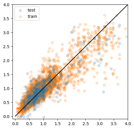
mlp.fit(X_train, y_train)
y_pred = mlp.predict(X_test)
y_pred0 = mlp.predict(X_train)
mse = mean_squared_error(y_test, y_pred)
print("MSE:", mse)
fig, ax = plt.subplots(figsize=(5,5))
ax.scatter(y_test, y_pred, alpha=0.2, label="test")
ax.scatter(y_train, y_pred0, alpha=0.2, label='train', zorder = -1)
ax.plot([0, 4], [0, 4], color='black')
#ax.set_xlabel(“z_spec”)
#ax.set_ylabel(“z_pred”)
ax.set_xlim(-0.1, 4)
ax.set_ylim(-0.1, 4)
ax.legend()
plt.show()
MSE: 0.14376234464783927