Python: An Introduction to Numpy#
Python language is an excellent tool for general-purpose programming, with a highly readable syntax, rich and powerful data types (strings, lists, sets, dictionaries, arbitrary length integers, etc) and a very comprehensive standard library.
However, Python was not designed specifically for mathematical and scientific computing. In its design, Python does not have facilities for the efficient representation of multidimensional datasets, tools for linear algebra and general matrix manipulations, nor any data visualization facilities.
In contrast, much of modern scientific computing has been built on top of libraries written in the Fortran language, which has native support for vectors and matrices as well as a library of mathematical functions that can efficiently operate on entire arrays at once.
Numpy aims at filling some of the numerical operation needs. It is actually build around the Scipy ecosystem.
Import numpy as np#
One can install numpy with pip:
pip install numpy
A common line in many scientific scripts is importing Numpy as
import numpy as np
This alias (using as) is convenient to shorten how many letters we need to type since Numpy is used so many times.
Basics of Numpy arrays#
One of the major advancement of numpy resides in its arrays.
The Numpy array structure#
NumPy provides an N-dimensional array type, the ndarray, which describes a collection of “items” of the same type. This means every item takes up the same size block or memory and all blocks are interpreted in the same manner: ndarrays are homogeneous, whether they contain integer, floats or more complex objects.
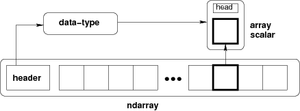
Conceptually, an ndarray is the combination of three fundamental objects used to describe the data in memory:
the data in consecutive memory blocks, and the data-type object that describes the layout of a single fixed-size element of the array. When one access an element of the array, Python returns a Python scalar object.
As mentioned above, the main object provided by numpy is a powerful array. We’ll start by exploring how the numpy array differs from Python lists.
Let start by creating a simple list and an array with the same contents of the list.
lst = [1, 2, 3, 4, 5, 6]
arr = np.array([1, 2, 3, 4, 5, 6])
Element indexing#
Elements of a one-dimensional array are accessed with the same syntax as a list:
lst[0], arr[0], lst[-1], arr[-1]
(1, 1, 6, 6)
lst[:4], arr[:4]
([1, 2, 3, 4], array([1, 2, 3, 4]))
Note that python represents the array slightly differently than a list: array([...]).
The first difference to note between lists and arrays is that arrays are homogeneous; i.e. all elements of an array must be of the same type. In contrast, lists can contain elements of arbitrary type. For example, we can change the last element in our list above to be a string:
lst[-1] = 'a string'
lst
[1, 2, 3, 4, 5, 'a string']
but the same can not be done with an array, as we get an error message:
arr[-1] = 'a string'
---------------------------------------------------------------------------
ValueError                                Traceback (most recent call last)
Cell In[6], line 1
----> 1 arr[-1] = 'a string'

ValueError: invalid literal for int() with base 10: 'a string'
The information about the type of the data in an array is contained in its dtype attribute
arr.dtype
dtype('int64')
Once an array has been created, its dtype is fixed and it can only store elements of the same type.
arr[-1] = 10
arr
array([ 1, 2, 3, 4, 5, 10])
What happens if we change add a different numerical type?
arr[-1] = 3.1415
arr
array([1, 2, 3, 4, 5, 3])
Implicitly Python attempts to cast the value using dtype, it does not change the type automatically.
arr.dtype.type(3.1415)
3
Creating Arrays#
Above we created one array from an existing list. There are multiple other ways. A common need is to have an array initialized with a constant value, and very often this value is 0 or 1 (suitable as starting value for additive and multiplicative loops respectively); zeros creates arrays of all zeros, with any desired dtype:
np.zeros(5, dtype=float)
array([0., 0., 0., 0., 0.])
np.zeros(5, dtype=int)
array([0, 0, 0, 0, 0])
np.zeros(3, dtype=complex)
array([0.+0.j, 0.+0.j, 0.+0.j])
print('5 ones:', np.ones(5))
5 ones: [1. 1. 1. 1. 1.]
By default, Numpy creates float arrays (i.e. double precision floats)
If we want an array initialized with an arbitrary value, np.empty creates such an array, you can then use the np.fill method to put the value we want into the array:
a = np.empty(4, dtype=int)
a.fill(42)
a
array([42, 42, 42, 42])
Numpy also offers the arange function, which works like the builtin range but returns an array instead of a list:
print(np.arange(5))
print(np.arange(3, 6, 0.5))
[0 1 2 3 4]
[3.  3.5 4.  4.5 5.  5.5]
and the linspace and logspace functions to create linearly and logarithmically-spaced grids respectively, with a fixed number of points and including both ends of the specified interval:
print(np.linspace(0, 1, 4))
print(np.logspace(0, 3, 4))
[0.         0.33333333 0.66666667 1.        ]
[   1.   10.  100. 1000.]
Finally, it is often useful to create arrays with random numbers that follow a specific distribution. The np.random module contains functions that can be used to this effect.
print(np.random.randn(5))
print(np.random.uniform(0, 10, size=5))
print(np.random.normal(5, 1, size=5))
[ 1.00575995 -1.10020353  1.06996585  1.42384826  0.44498963]
[4.83165679 9.47196466 4.85249266 7.12540851 0.9830064 ]
[4.04135044 5.39045932 5.74068594 6.334547   6.59903963]
Arrays with more than one dimension#
Up until now all our examples have used one-dimensional arrays. But Numpy can create arrays of aribtrary dimensions, and all the previous methods work similarly.
lst2 = [[1, 2], [3, 4]]
arr2 = np.array([[1, 2], [3, 4]])
print(lst2)
arr2
[[1, 2], [3, 4]]
array([[1, 2],
       [3, 4]])
With two-dimensional arrays we start seeing the benefit of Numpy. While a nested list can be indexed using repeatedly the [ ] operator, multidimensional arrays support a much more natural indexing syntax with a single [ ] and a set of indices separated by commas
print(lst2[0][1])
print(arr2[0][1], arr2[0,1])
2
2 2
Most of the array creation functions listed above can be used with more than one dimension, for example:
np.zeros((2,3)), np.ones((2,2)), np.random.normal(10, 3, (2, 4))
(array([[0., 0., 0.],
        [0., 0., 0.]]),
 array([[1., 1.],
        [1., 1.]]),
 array([[17.57850522,  6.40006379, 15.26014135,  9.12044918],
        [11.40844105,  5.7175767 ,  6.192082  , 13.85750891]]))
In fact, numpy offers functions to change the shape of an array at any time (reshape), as long as the total number of elements is unchanged.
np.arange(8).reshape(2, 4)
array([[0, 1, 2, 3],
       [4, 5, 6, 7]])
Numpy views and not copies#
Numpy is also very memory efficient in most of its operations. Reshaping (like most numpy operations) provides a view of the same memory:
arr = np.arange(8)
arr2 = arr.reshape(2, 4)
# changing a value in arr affects arr2
arr[0] = 1000
print(arr)
print(arr2)
[1000    1    2    3    4    5    6    7]
[[1000    1    2    3]
 [   4    5    6    7]]
This lack of copying allows for very efficient vectorized operations.
x = np.random.rand(5, 2)
print(x)
print(x.transpose())
[[0.34199477 0.58804653]
 [0.17521856 0.0355019 ]
 [0.21917783 0.17360486]
 [0.21308281 0.36500134]
 [0.77306321 0.66779829]]
[[0.34199477 0.17521856 0.21917783 0.21308281 0.77306321]
 [0.58804653 0.0355019  0.17360486 0.36500134 0.66779829]]
Slices#
With multidimensional arrays, it is sometimes useful to extract patches, chunks, and entire dimensions. To do this, Numpy provides a slicing mechanism, and you can mix and match slices and single indices in the different dimensions.
arr = arr = np.arange(8).reshape(2, 4)
print('Slicing in the second row:', arr[1, 2:4])
print('All rows, third column   :', arr[:, 2])
print('First row:  ', arr[0])
print('Second row: ', arr[1])
Slicing in the second row: [6 7]
All rows, third column   : [2 6]
First row:   [0 1 2 3]
Second row:  [4 5 6 7]
Array Properties and Methods#
As an array is a collection of values that can be manipulated, it is important to know the properties and methods of a Numpy array.
Array Shapes, dimensions, types#
As you just saw above, arrays can be of any dimension, shape and size you desire. In fact, there are three main array attributes you need to know to work out the characteristics of an array:
.ndim: the number of dimensions of an array.shape: the number of elements in each dimension (like callinglen()on each dimension).size: the total number of elements in an array (i.e., the product of.shape).dtype: the data type of an array.nbytes: the total number of bytes in an array, which depends on the data type.
# for convenience
def print_array(x):
    print(f"Dimensions: {x.ndim}")
    print(f"     Shape: {x.shape}")
    print(f"      Size: {x.size} elements")
    print(f"    Memory: {x.nbytes} Bytes")
    print(f" Data type: {x.dtype}")
    print("")
    print(x)
print_array(np.ones(3))
Dimensions: 1
     Shape: (3,)
      Size: 3 elements
    Memory: 24 Bytes
 Data type: float64

[1. 1. 1.]
print_array(np.ones((3, 2)))
Dimensions: 2
     Shape: (3, 2)
      Size: 6 elements
    Memory: 48 Bytes
 Data type: float64

[[1. 1.]
 [1. 1.]
 [1. 1.]]
print_array(np.ones((1, 2, 3, 4), dtype=int))
Dimensions: 4
     Shape: (1, 2, 3, 4)
      Size: 24 elements
    Memory: 192 Bytes
 Data type: int64

[[[[1 1 1 1]
   [1 1 1 1]
   [1 1 1 1]]

  [[1 1 1 1]
   [1 1 1 1]
   [1 1 1 1]]]]
Above 3 dimensions, printing arrays starts to be challenging.
Arrays also have many useful methods, some especially useful ones are:
print('Minimum and maximum             :', arr.min(), arr.max())
print('Sum and product of all elements :', arr.sum(), arr.prod())
print('Mean and standard deviation     :', arr.mean(), arr.std())
Minimum and maximum             : 0 7
Sum and product of all elements : 28 0
Mean and standard deviation     : 3.5 2.29128784747792
For these methods, you can often apply it to a single dimension instead of on all the elements of the array using the axis parameter; for example:
print('Our array `arr`:\n', arr)
print('The sum of elements along the rows is    :', arr.sum(axis=1))
print('The sum of elements along the columns is :', arr.mean(axis=0))
Our array `arr`:
 [[0 1 2 3]
 [4 5 6 7]]
The sum of elements along the rows is    : [ 6 22]
The sum of elements along the columns is : [2. 3. 4. 5.]
Another widely used operation on arrays is the transposition, which Numpy provides a shortcut for as a .T attribute:
arr, arr.T
(array([[0, 1, 2, 3],
        [4, 5, 6, 7]]),
 array([[0, 4],
        [1, 5],
        [2, 6],
        [3, 7]]))
Exercise: Explore some of the following attributes/methods on your own:
    arr.T             arr.copy          arr.getfield      arr.put           arr.squeeze
    arr.all           arr.ctypes        arr.imag          arr.ravel         arr.std
    arr.any           arr.cumprod       arr.item          arr.real          arr.strides
    arr.argmax        arr.cumsum        arr.itemset       arr.repeat        arr.sum
    arr.argmin        arr.data          arr.itemsize      arr.reshape       arr.swapaxes
    arr.argsort       arr.diagonal      arr.max           arr.resize        arr.take
    arr.astype        arr.dot           arr.mean          arr.round         arr.tofile
    arr.base          arr.dtype         arr.min           arr.searchsorted  arr.tolist
    arr.byteswap      arr.dump          arr.nbytes        arr.setasflat     arr.tostring
    arr.choose        arr.dumps         arr.ndim          arr.setfield      arr.trace
    arr.clip          arr.fill          arr.newbyteorder  arr.setflags      arr.transpose
    arr.compress      arr.flags         arr.nonzero       arr.shape         arr.var
    arr.conj          arr.flat          arr.prod          arr.size          arr.view
    arr.conjugate     arr.flatten       arr.ptp           arr.sort
Operations with arrays#
Arrays support all regular arithmetic operators, and the numpy library also contains a complete collection of basic mathematical functions that operate on arrays.
All operations with arrays are commonly applied element-wise, i.e., are applied to all the elements of the array at the same time.
arr1 = np.arange(4)
arr2 = np.arange(10, 14)
print(arr1, '+', arr2, '=', arr1+arr2)
[0 1 2 3] + [10 11 12 13] = [10 12 14 16]
Importantly, * the multiplication operator is by default applied element-wise, it is not the matrix multiplication from linear algebra (this is @ operator):
print(arr1, '*', arr2, '=', arr1*arr2)
print("10 * arr1 =", 10 * arr1)
[0 1 2 3] * [10 11 12 13] = [ 0 11 24 39]
10 * arr1 = [ 0 10 20 30]
the dot product of two vectors is using the @ operator in python (.* in matlab)
arr1 @ arr2
74
Broadcasting#
In principle, array operations (e.g., mutiplication or addition) must math in their dimensionality. However, Numpy will match the dimensions when possible by “broadcasting” the dimensions when possible.
print(np.arange(12).reshape((3, 4)) + np.arange(4))
[[ 0  2  4  6]
 [ 4  6  8 10]
 [ 8 10 12 14]]
However, it is not always obvious to Numpy:
print(np.arange(12).reshape((3, 4)) + np.arange(3))
---------------------------------------------------------------------------
ValueError                                Traceback (most recent call last)
Cell In[37], line 1
----> 1 print(np.arange(12).reshape((3, 4)) + np.arange(3))

ValueError: operands could not be broadcast together with shapes (3,4) (3,)
In this example, we need to help Numpy to create the missing dimension at the right place.
Rules of Broadcasting#
Broadcasting rules can do the following:
If the two arrays differ in their number of dimensions, the shape of the array with fewer dimensions is padded with ones on its leading (left) side.
If the shape of the two arrays does not match in any dimension, the array with shape equal to 1 in that dimension is stretched to match the other shape.
If in any dimension the sizes disagree and neither is equal to 1, an error is raised.
Note
Numpy does not copy any data in memory during broadcasting! This broadcasting behavior is in practice enormously powerful, especially because when numpy broadcasts to create new dimensions or to ‘stretch’ existing ones, it doesn’t actually replicate the data. This can save lots of memory in cases when the arrays in question are large and can have significant performance implications.
Visualizing Broadcasting#
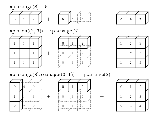
Fig. 4 The light boxes represent the broadcasted values: again, this extra memory is not actually allocated in the course of the operation, but it can be useful conceptually to imagine that it is. Credit: Jake VanderPlas image source#
Other common element-wise Functions#
Numpy ships with a full complement of mathematical functions that work on entire arrays, including logarithms (log, log10), exponentials (exp), trigonometric (cos, sin, atan) and hyperbolic trigonometric functions, etc. Furthermore, scipy ships a rich special function library in the scipy.special module that includes Bessel, Airy, Fresnel, Laguerre and other classical special functions. For example, sampling the sine function at 100 points between \(0\) and \(2\pi\) is as simple as:
x = np.linspace(0, 2 * np.pi, 100)
y = np.sin(x)
Linear algebra in numpy#
As scientists, we often need to do some linear algebra operations on our arrays. Numpy ships with a linear algebra library.
For instance, the scalar dot product when its arguments are vectors (one-dimensional arrays) and the traditional matrix multiplication when one or both of its arguments are two-dimensional arrays:
v1 = np.array([1, 2, 3])
v2 = np.array([1, 0, 1])

# note the various ways to write the same operation.
print(v1, '.', v2, '= (np.dot(v1, v2)) =', np.dot(v1, v2))
print(v1, '.', v2, '=     (v1.dot(v2)) =', v1.dot(v2))
print(v1, '.', v2, '=       (v1 @ v2)  =', v1 @ v2)
[1 2 3] . [1 0 1] = (np.dot(v1, v2)) = 4
[1 2 3] . [1 0 1] =     (v1.dot(v2)) = 4
[1 2 3] . [1 0 1] =       (v1 @ v2)  = 4
We can also do products of matrices and vectors.
In the above, the array v1 should be viewed as a column vector in traditional linear algebra notation; numpy makes no distinction between row and column vectors (these are one dimensional arrays). It simply verifies that the dimensions match the required rules of matrix multiplication.
A = np.arange(6).reshape(2, 3)
v = np.arange(3)
print("A = ", A )
print("v = ", v )
print("")
print("A @ v1 =", A @ v1)
print("A.T @ A =", A.T @ A)
A =  [[0 1 2]
 [3 4 5]]
v =  [0 1 2]

A @ v1 = [ 8 26]
A.T @ A = [[ 9 12 15]
 [12 17 22]
 [15 22 29]]
Furthermore, the numpy.linalg module includes additional functionality such as determinants, matrix norms, Cholesky decompositions, eigenvalue and singular value decompositions, etc. For even more linear algebra tools, scipy.linalg contains the majority of the tools in the classic LAPACK libraries as well as functions to operate on sparse matrices.
Exercise 1: Numerical integration with trapezoidal rule#
In this exercise, you are tasked with implementing the simple trapezoid rule formula for numerical integration to compute the definite integral
The rule is to partition the interval \([a,b]\) into smaller subintervals, and then approximate the area under the curve for each subinterval by the area of a trapezoid.

Fig. 5 Source: wikipedia.org#
By subdividing the interval \([a,b]\), the area under \(f(x)\) can thus be approximated as the sum of the areas of all the resulting trapezoids.
If we denote by \(x_{i}\) (\(i=0,\ldots,n,\) with \(x_{0}=a\) and \(x_{n}=b\)) the abscissas where the function is sampled, then
The common case of using equally spaced abscissas with spacing \(h=(b-a)/n\) reads simply
One frequently receives the function values already precomputed, \(y_{i}=f(x_{i}),\) so the equation above becomes
Q1: Write a function trapz(x, y), that applies the trapezoid formula to pre-computed values, where x and y are 1-d arrays (Use numpy operations, not loops!). Check your code on \(\int_0^3 x^2 dx\).
Show code cell source
def trapz(x: np.ndarray, y: np.ndarray) -> np.ndarray:
    """Trapezoidal rule"""
    return np.sum(0.5 * (y[1:] + y[:-1]) * (x[1:] - x[:-1]))

# math:
true_value = 1./3. * (3 ** 3 - 0 ** 3)

x = np.arange(0, 3, 0.001)
Fx = trapz(x, x ** 2)
print('expected value', true_value)
print('    user trapz', Fx)
print('         error', Fx - true_value)
expected value 9.0
    user trapz 8.991003499500001
         error -0.008996500499998561
Q2: Compare with math and with np.trapz
Show code cell source
x = np.arange(0, 3, 0.001)
Fx = trapz(x, x ** 2)
npFx = np.trapz(x ** 2, x)
print('expected value', true_value)
print('    user trapz', Fx)
print('      np.trapz', npFx)
print('    difference', npFx - Fx)
expected value 9.0
    user trapz 8.991003499500001
      np.trapz 8.991003499500001
    difference 0.0
Important
scipy.integrate contains plenty integration methods.