Predicting galaxy redshifts from 3D-HST

Last update June, 13 2023

Setup environment

%%file requirements.txt
matplotlib
pandas
numpy
scikit-learn
tensorflow
torch
jax
jaxlib
flax
astropy
plotly
git+https://github.com/mfouesneau/ezdata

Overwriting requirements.txt

!python3 -m pip install -q -r requirements.txt

Notebook setup

%matplotlib inline
import pandas as pd
import numpy as np
import pylab as plt
from IPython.display import Markdown, display
from ezdata.matplotlib import light_minimal
plt.style.use(light_minimal)

Predicting galaxy redshift via regression on 3D-HST photometry

Download data

First, download the 3D-HST catalog from the MAST archive. This dataset is described in Skelton et. al 2014.

from astropy.utils.data import download_file
import tarfile
import os


if not os.path.isdir('3dhst_master.phot.v4.1'):
    file_url = 'https://archive.stsci.edu/missions/hlsp/3d-hst/RELEASE_V4.0/Photometry/3dhst_master.phot.v4.1.tar'
    tarfile.open(download_file(file_url, cache=True), "r:")\
           .extract('3dhst_master.phot.v4.1/3dhst_master.phot.v4.1.cat', '.')
else:
    print('file already downloaded.')

file already downloaded.

Read the combined photmetric catalog into a dataframe via astropy

import pandas as pd
fname = '3dhst_master.phot.v4.1/3dhst_master.phot.v4.1.cat'
with open(fname, 'r') as fin:
    header = fin.readline()[1:]  #remove comment character
    df = pd.read_csv(fin, names=header.strip().split(), comment='#', delimiter='\s+')
df = df.set_index('id')

df

	field	ra	dec	x	y	z_spec	z_peak	faper_F140W	eaper_F140W	faper_F160W	...	flags	f140w_flag	star_flag	use_phot	near_star	nexp_f125w	nexp_f140w	nexp_f160w	lmass	Av
id
1.0	AEGIS	215.222382	53.004185	9590.50	3057.30	-1.0000	0.0100	-82.0410	-82.041000	22531.00000	...	0	0	1	0	0	2	0	3	7.51	1.1
2.0	AEGIS	215.096588	52.918053	16473.20	3150.20	-1.0000	0.0100	3.5078	0.074233	3.99050	...	3	0	0	0	0	4	4	4	5.62	0.1
3.0	AEGIS	215.161469	52.959461	13060.10	2982.30	-1.0000	0.2062	-1.9043	-1.904300	1.38110	...	1	0	0	1	0	2	0	2	9.00	1.1
4.0	AEGIS	215.305298	53.052921	5422.80	2692.10	-1.0000	0.0355	-72.3250	-72.325000	0.82549	...	0	0	0	0	0	1	0	1	4.78	0.4
5.0	AEGIS	215.041840	52.871273	19894.60	2834.40	-1.0000	0.3427	1890.5000	0.133300	-99.00000	...	0	1	2	0	1	0	3	0	11.57	0.5
...	...	...	...	...	...	...	...	...	...	...	...	...	...	...	...	...	...	...	...	...	...
44098.0	UDS	34.363106	-5.122067	14578.84	11076.42	-1.0000	0.1852	188.8200	0.170750	-99.00000	...	0	1	2	0	0	0	3	0	10.21	0.2
44099.0	UDS	34.333569	-5.123219	16343.92	11007.12	-1.0000	0.6716	1.7193	0.129080	-99.00000	...	0	1	2	0	0	0	3	0	8.49	0.7
44100.0	UDS	34.363682	-5.123123	14544.39	11013.01	1.4196	2.7489	1.3829	0.113830	-99.00000	...	0	1	2	0	0	0	4	0	9.08	1.4
44101.0	UDS	34.556389	-5.123040	3028.23	11017.04	-1.0000	1.1716	-99.0000	-99.000000	5.51670	...	1	0	0	0	0	1	0	2	10.55	1.0
44102.0	UDS	34.365097	-5.121975	14459.90	11081.91	-1.0000	0.6160	1.5335	0.152730	-99.00000	...	0	1	2	0	0	0	3	0	8.58	0.0

207967 rows × 37 columns

Exploring the dataset

Now we will examine the contents of the catalog.

The dataset contains standard information such as target id, field name, coordinates (ra, dec), fluxes, uncertainties, and various photometric flags (see Skelton et. al 2014, or download the README here).

In addition, there are some derived properties such as photometric redshift (z_peak), spectroscopic redshift (z_spec), mass (lmass) and dust extinction in the V band (Av).

Kriek et al (2018; FAST) describe the masse estimates.

Keep in mind that we are interested in predicting redshift, so our “target” variable will be z_spec. The “features” will be all relevant columns.

df.columns

Index(['field', 'ra', 'dec', 'x', 'y', 'z_spec', 'z_peak', 'faper_F140W',
       'eaper_F140W', 'faper_F160W', 'eaper_F160W', 'f_F606W', 'e_F606W',
       'f_F814W', 'e_F814W', 'f_F125W', 'e_F125W', 'f_F140W', 'e_F140W',
       'f_F160W', 'e_F160W', 'tot_cor', 'kron_radius', 'a_image', 'b_image',
       'flux_radius', 'fwhm_image', 'flags', 'f140w_flag', 'star_flag',
       'use_phot', 'near_star', 'nexp_f125w', 'nexp_f140w', 'nexp_f160w',
       'lmass', 'Av'],
      dtype='object')

Cleaning the dataset

For our application, there are columns that we do not / should not use in making a model of redshift. Let’s consider the following comments:

• we will drop the identifier, the field, x, y, ra, dec because we do not need to learn any anisotropy due to a limited survey.

• we consider all fluxes, but note that the faper_ fields correspond to somewhat duplicated measurements. Let’s drop the latter fields.

• nexp_ gives us the number of exposures, which does not seem important here.

• tot_cor corresponds to a flux (aperture) correction.

• kron_radius, corresponds to a KRON radius, i.e. 90% of the flux contained in an aperture size twice that radius. flux_radius similarly corresponds to the half light radius. Let’s remove those.

• a_image & b_image correspond to semi-major and semi-minor axes

• fwhm_image corresponds to the Gaussian fit of the objects’ cores. Not relevant for us.

• star_flag if 0, corresponds to galaxy. Any other value means star.

• lmass corresponds to the estimated mass of the quasar based on the redshift and luminosity. We must remove it to avoid data leakage.

• Av corresponds to the extinction along the line of sight. This may be helpful to keep to tell us about the reddening and dimming of a source.

• use_phot & near_star are flags about the detection and measurements. These could be interesting to use to get the best training set possible.

df.describe()

	ra	dec	x	y	z_spec	z_peak	faper_F140W	eaper_F140W	faper_F160W	eaper_F160W	...	flags	f140w_flag	star_flag	use_phot	near_star	nexp_f125w	nexp_f140w	nexp_f160w	lmass	Av
count	207967.000000	207967.000000	207967.000000	207967.000000	207967.000000	207967.000000	207967.000000	207967.000000	207967.000000	207967.000000	...	207967.000000	207967.000000	207967.000000	207967.000000	207967.000000	207967.000000	207967.000000	207967.000000	207967.000000	207967.000000
mean	122.067472	14.465094	12156.481048	10233.742518	-0.953653	1.177393	-15.424237	-22.113783	13.392734	-0.518764	...	0.500642	0.003303	1.310165	0.847005	0.044267	8.358509	4.425048	9.051638	8.410625	0.318929
std	73.831227	35.387678	7233.913627	5733.813482	0.489124	6.727479	323.776749	54.457811	596.100221	7.605170	...	1.278831	0.057380	0.943662	0.359984	0.205687	10.919348	9.310295	15.192599	1.511090	0.544946
min	34.216633	-27.959742	7.400000	1273.020000	-99.900000	-99.000000	-482.630000	-482.630000	-99.000000	-99.000000	...	0.000000	0.000000	0.000000	0.000000	0.000000	0.000000	0.000000	0.000000	-1.000000	-1.000000
25%	53.061646	-5.272032	7316.685000	6161.300000	-1.000000	0.817400	-48.633500	-48.633500	0.186090	0.026516	...	0.000000	0.000000	0.000000	1.000000	0.000000	4.000000	0.000000	4.000000	7.910000	0.000000
50%	150.091034	2.274822	10578.100000	8873.450000	-1.000000	1.415900	0.178810	0.069309	0.355380	0.035040	...	0.000000	0.000000	2.000000	1.000000	0.000000	4.000000	4.000000	4.000000	8.500000	0.100000
75%	189.306900	52.957975	15137.135000	13184.660000	-1.000000	2.128050	0.491190	0.086337	0.939190	0.042530	...	0.000000	0.000000	2.000000	1.000000	0.000000	8.000000	4.000000	8.000000	9.180000	0.500000
max	215.305298	62.388302	37668.900000	30753.300000	6.118000	5.960900	47052.000000	10592.000000	91185.000000	474.560000	...	23.000000	1.000000	2.000000	1.000000	1.000000	91.000000	84.000000	132.000000	14.630000	4.000000

8 rows × 36 columns

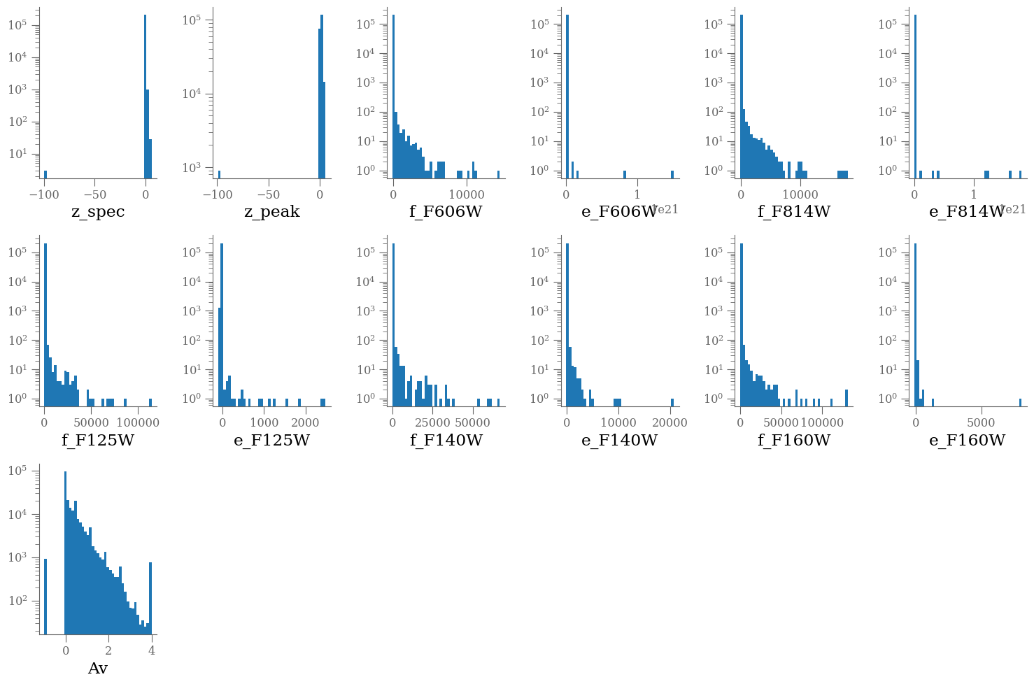
Looking at the values, we see that some zspec, fluxes and Av values are negative, some fluxes are set to -99.0

remove = ['field', 'ra', 'dec', 'x', 'y',
          'faper_F140W', 'eaper_F140W', 'faper_F160W', 'eaper_F160W',
          'tot_cor', 'kron_radius', 'a_image', 'b_image',
          'flux_radius', 'fwhm_image', 'flags', 'f140w_flag', 'star_flag',
          'use_phot', 'near_star', 'nexp_f125w', 'nexp_f140w', 'nexp_f160w',
          'lmass']

columns = [k for k in df.columns if k not in remove]

wrap = 6

plt.figure(figsize=(15, 10))

nlines = len(columns) // wrap +  int(len(columns) % wrap > 0) 

for e, colname in enumerate(columns, 1):
    plt.subplot(nlines, wrap, e)
    plt.hist(df[colname], bins=43, log=True)
    plt.xlabel(colname)

plt.tight_layout()

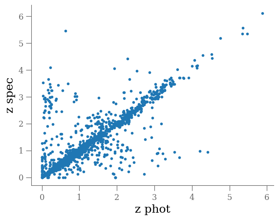
select = (df.z_peak > 0) & (df.z_spec > 0)
plt.plot(df[select].z_peak, df[select].z_spec, '.', rasterized=True)
plt.xlabel('z phot')
plt.ylabel('z spec')

Text(0, 0.5, 'z spec')

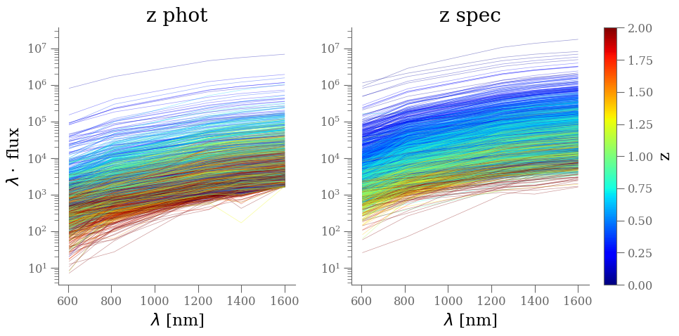
flux_cols = [name for name in df.columns if name.startswith('f_F')]
positive_flux = ' & '.join([f'({col:s} > 0)' for col in flux_cols])
x_ = np.array([606, 814, 1250, 1400, 1600])

select_zphot = '(star_flag == 0) & (use_phot == 1) & (z_peak > 0)'
select_zspec = '(star_flag == 0) & (z_spec > 0)'

cmap = plt.get_cmap('jet')
norm = plt.Normalize(vmin=0, vmax=2)


plt.figure(figsize=(10, 5))

ax = plt.subplot(121)
select = df.eval(select_zphot + '&' + positive_flux)
df_ = df[select]
ind = np.random.choice(len(df_), 2_000, replace=False)
X = df_[flux_cols].to_numpy()[ind]
y = df_['z_peak'].to_numpy()[ind]

for xk, yk in zip(X, y):
    color = cmap(norm(yk))
    plt.plot(x_, x_ * xk, color=color, rasterized=True, alpha=0.4, lw=0.5)

plt.yscale('log')
sm = plt.cm.ScalarMappable(cmap=cmap, norm=norm)
sm.set_array([])
cbar = plt.colorbar(sm, ax=plt.gca())
cbar.set_label('z phot')
cbar.ax.set_visible(False)
plt.ylabel('$\lambda  \cdot $ flux')
plt.xlabel('$\lambda$ [nm]')
plt.title('z phot')


plt.subplot(122,  sharex=ax, sharey=ax)
select = df.eval(select_zspec + '&' + positive_flux)
df_ = df[select]
ind = np.random.choice(len(df_), 2_000, replace=False)
X = df_[flux_cols].to_numpy()[ind]
y = df_['z_spec'].to_numpy()[ind]
for xk, yk in zip(X, y):
    color = cmap(norm(yk))
    plt.plot(x_, x_ * xk, color=color, rasterized=True, alpha=0.4, lw=0.5)
plt.yscale('log')
sm = plt.cm.ScalarMappable(cmap=cmap, norm=norm)
sm.set_array([])
cbar = plt.colorbar(sm, ax=plt.gca())
cbar.set_label('z')
plt.title('z spec')

plt.xlabel('$\lambda$ [nm]')

plt.tight_layout()

remove = ['field', 'ra', 'dec', 'x', 'y',
          'faper_F140W', 'eaper_F140W', 'faper_F160W', 'eaper_F160W',
          'tot_cor', 'kron_radius', 'a_image', 'b_image',
          'flux_radius', 'fwhm_image', 'flags', 'f140w_flag', 'star_flag',
          'use_phot', 'near_star', 'nexp_f125w', 'nexp_f140w', 'nexp_f160w',
          'lmass']

flux_cols = [name for name in df.columns if name.startswith('f_F')]

positive_flux = ' & '.join([f'({col:s} > 0)' for col in flux_cols])

select_zphot = '(star_flag == 0) & (use_phot == 1) & (z_peak > 0) & (Av >= 0)'
select_zspec = '(star_flag == 0) & (z_spec > 0) & (Av >= 0)'

select = df.eval(select_zspec + '&' + positive_flux)
df_ = df[select].reset_index()
target = 'z_spec'
# features = [col for col in df_ if col not in remove + ['z_spec', 'z_peak'] ]
features = flux_cols + ['Av']

Markdown(f"""
**features** {features}

**target**: {target} """)

features [‘f_F606W’, ‘f_F814W’, ‘f_F125W’, ‘f_F140W’, ‘f_F160W’, ‘Av’]

target: z_spec

df_x = pd.concat([df_[[fk for fk in features if fk not in flux_cols]], 
                  np.log10(df_[flux_cols]).rename(columns={k: k.replace('f_', 'm_') for k in flux_cols})], 
                  axis=1)
df_y = df_[target]

df_x

	Av	m_F606W	m_F814W	m_F125W	m_F140W	m_F160W
0	0.1	0.797247	0.975064	1.086893	1.152105	1.172282
1	1.2	0.686877	0.881835	1.191004	1.271934	1.350558
2	0.6	0.997478	1.173245	1.281374	1.307410	1.333185
3	0.1	0.537932	1.090822	1.508880	1.572964	1.636698
4	0.7	1.157608	1.335598	1.491544	1.531849	1.576698
...	...	...	...	...	...	...
2287	0.6	0.310247	1.097466	1.719588	1.794063	1.881316
2288	0.6	2.120245	2.233580	2.333165	2.319252	2.425632
2289	0.6	0.960361	1.216166	1.435717	1.483602	1.520156
2290	1.4	2.104111	2.280373	2.507032	2.561006	2.613112
2291	0.7	1.553167	1.690878	1.855410	1.884246	1.910507

2292 rows × 6 columns

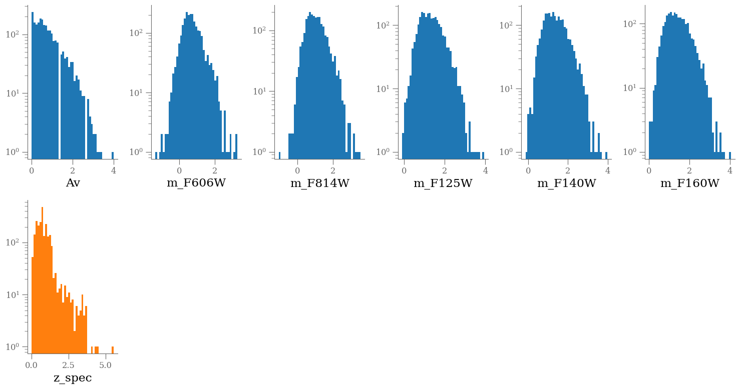
columns = [k for k in df_x.columns]

wrap = 6

nlines = (len(columns) + 1) // wrap +  int((len(columns) + 1) % wrap > 0)

plt.figure(figsize=(15, nlines * 4))
for e, colname in enumerate(columns, 1):
    plt.subplot(nlines, wrap, e)
    plt.hist(df_x[colname], bins=43, log=True)
    plt.xlabel(colname)

plt.subplot(nlines, wrap, e + 1)
plt.hist(df_y, bins=43, log=True, color='C1')
plt.xlabel(target)

plt.tight_layout()

Divide the data into train, test and validation sets

Note that typically one needs to pass arrays to the common libraries.

X = df[features].values
y = df[target].values

However, Scikit-learn has implemented pandas interfaces, so we do not need to do so in this particular exercise.

Divide the data into train, validation and test sets. We will use the following definitions:

• Training: The data used to update model parameters (e.g., coefficients or matrix element values).

• Validation: The data used to update model selection (for instance, we might change hyperparameters of a model based on the validation metrics).

• Testing: The data used to make final predictions, and possibly evaluate the final model score.

from sklearn.model_selection import train_test_split

# first reserve 70% of the data for training, 30% for validation
X_train, X_test, y_train, y_test = train_test_split(df_x, df_y, test_size=0.3, random_state=42)

Explore regression models

Here we explore a few options for regressor models.

Linear Regression

Let’s do a simple one first

from sklearn.linear_model import LinearRegression

lin = LinearRegression()
lin.fit(X_train, y_train)

LinearRegression()

In a Jupyter environment, please rerun this cell to show the HTML representation or trust the notebook.
On GitHub, the HTML representation is unable to render, please try loading this page with nbviewer.org.

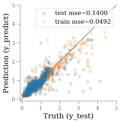
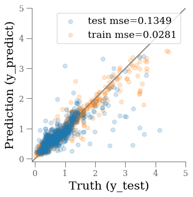
To quantify the performance of the model, we will apply it to the validation set and compare the predicted values with the true values by computing the mean squared error:

from sklearn.metrics import mean_squared_error

y_predict = lin.predict(X_test)
y_predict0 = lin.predict(X_train)
mse_train = mean_squared_error(y_train, y_predict0)
mse_test = mean_squared_error(y_test, y_predict)

fig, ax = plt.subplots(1, 1, figsize=(4, 4))
ax.scatter(y_test, y_predict, alpha=0.2, label=f'test mse={mse_test:0.4f}')
ax.scatter(y_train, y_predict0, alpha=0.2, label=f'train mse={mse_train:0.4f}', zorder=-1)
ax.plot(ax.get_xlim(), ax.get_xlim(), zorder=-1, color='0.5')
ax.set_aspect('equal')
ax.set_xlim(-0.1, 5)
ax.set_ylim(-0.1, 5)
ax.grid()
ax.set_xlabel('Truth (y_test)')
ax.set_ylabel('Prediction (y_predict)')
plt.legend(loc='upper left')

<matplotlib.legend.Legend at 0x7fe21b00bf70>

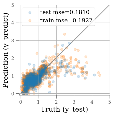
The MSE is not great. Not surprising given the simplicity of our model. Maybe we can do better changing the model?

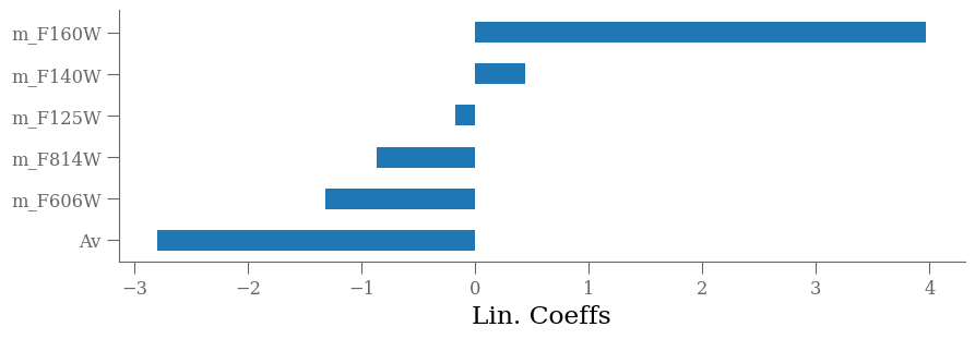
importances = lin.coef_
labels = lin.feature_names_in_
argsort = np.argsort(importances)
fig = plt.figure(figsize=[10, len(labels) * 0.5])
ax = fig.add_subplot(111)
ax.barh(np.arange(len(df_x.columns)), importances[argsort], 
        align='center', 
        height=0.5, 
        tick_label=labels)
ax.set_xlabel("Lin. Coeffs")

Text(0.5, 0, 'Lin. Coeffs')

from sklearn.pipeline import Pipeline
from sklearn.preprocessing import PolynomialFeatures, StandardScaler
from sklearn.linear_model import LassoLarsIC

pipe = Pipeline([
    ('polynomial', PolynomialFeatures(degree=3)),
    ('scaler', StandardScaler()),
    ('classifier', LassoLarsIC(normalize=True))
])

pipe.fit(X_train, y_train)

---------------------------------------------------------------------------
TypeError                                 Traceback (most recent call last)
Cell In[22], line 8
      2 from sklearn.preprocessing import PolynomialFeatures, StandardScaler
      3 from sklearn.linear_model import LassoLarsIC
      5 pipe = Pipeline([
      6     ('polynomial', PolynomialFeatures(degree=3)),
      7     ('scaler', StandardScaler()),
----> 8     ('classifier', LassoLarsIC(normalize=True))
      9 ])
     11 pipe.fit(X_train, y_train)

TypeError: __init__() got an unexpected keyword argument 'normalize'

y_predict = pipe.predict(X_test)
y_predict0 = pipe.predict(X_train)
mse_train = mean_squared_error(y_train, y_predict0)
mse_test = mean_squared_error(y_test, y_predict)

fig, ax = plt.subplots(1, 1, figsize=(4, 4))
ax.scatter(y_test, y_predict, alpha=0.2, label=f'test mse={mse_test:0.4f}')
ax.scatter(y_train, y_predict0, alpha=0.2, label=f'train mse={mse_train:0.4f}', zorder=-1)
ax.plot(ax.get_xlim(), ax.get_xlim(), zorder=-1, color='0.5')
ax.set_aspect('equal')
ax.set_xlim(-0.1, 5)
ax.set_ylim(-0.1, 5)
ax.grid()
ax.set_xlabel('Truth (y_test)')
ax.set_ylabel('Prediction (y_predict)')
plt.legend(loc='best')

<matplotlib.legend.Legend at 0x7f22c99c42b0>

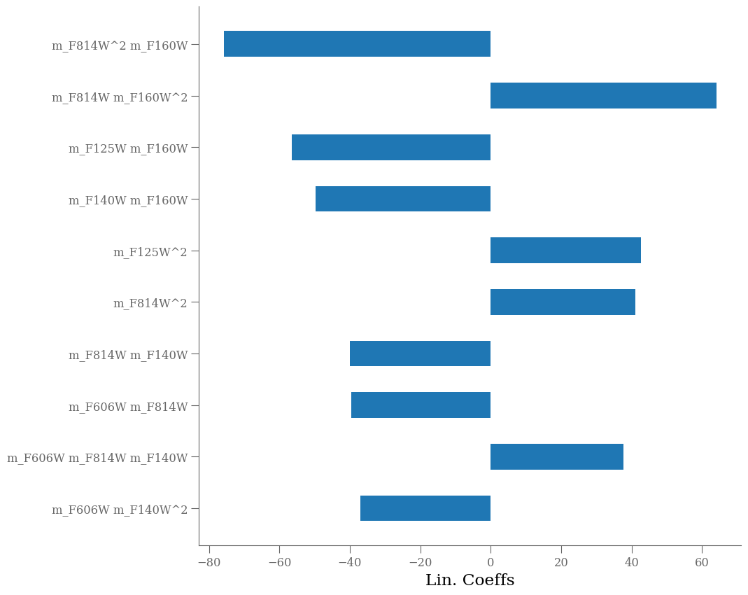
importances = pipe['classifier'].coef_
labels = pipe['polynomial'].get_feature_names_out()
argsort = np.argsort(np.abs(importances))[-10:]

importances = importances[argsort]
labels = labels[argsort]

fig = plt.figure(figsize=[10, 10])
ax = fig.add_subplot(111)
ax.barh(np.arange(len(labels)), importances, 
        align='center', 
        height=0.5, 
        tick_label=labels)
ax.set_xlabel("Lin. Coeffs")

Text(0.5, 0, 'Lin. Coeffs')

Other models

Using sklearn, it is very easy to change a model for something different.

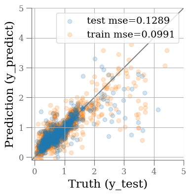
Random Forest

Using sklearn, we can very easily construct a decision tree model for regressing redshift from the photometric catalog features. A decision tree is composed of a series of if-else decision steps. The number of steps and the types of decision at each step is determined by training the algorithm with supervision. In this first example, we will use the DecisionTreeRegressor from sklearn.

from sklearn.ensemble import RandomForestRegressor

# use the same parameters as the Decision Tree
params = {
    "min_samples_split": 15,
    "min_samples_leaf": 5,
    "max_depth": 15,
}

# Initialize the model
rf = RandomForestRegressor(**params)

rf.fit(X_train, y_train)

RandomForestRegressor(max_depth=15, min_samples_leaf=5, min_samples_split=15)

In a Jupyter environment, please rerun this cell to show the HTML representation or trust the notebook.
On GitHub, the HTML representation is unable to render, please try loading this page with nbviewer.org.

y_predict = rf.predict(X_test)
y_predict0 = rf.predict(X_train)
mse_train = mean_squared_error(y_train, y_predict0)
mse_test = mean_squared_error(y_test, y_predict)

fig, ax = plt.subplots(1, 1, figsize=(4, 4))
ax.scatter(y_test, y_predict, alpha=0.2, label=f'test mse={mse_test:0.4f}')
ax.scatter(y_train, y_predict0, alpha=0.2, label=f'train mse={mse_train:0.4f}', zorder=-1)
ax.plot(ax.get_xlim(), ax.get_xlim(), zorder=-1, color='0.5')
ax.set_aspect('equal')
ax.set_xlim(-0.1, 5)
ax.set_ylim(-0.1, 5)
ax.set_xlabel('Truth (y_test)')
ax.set_ylabel('Prediction (y_predict)')
plt.legend(loc='best')

<matplotlib.legend.Legend at 0x7f22c96478b0>

The results are much improved by the random forest!

However, we must be cautious. It is possible that this model suffers from over-fitting. To visualize overfitting, we can compare the mean squared error (MSE) for models of increasing max_depth on the training and testing sets:

max_depths = np.arange(1, 20, 2).astype(int)

train_mse = []
test_mse = []

params = {
    "min_samples_split": 15,
    "min_samples_leaf": 5,
}

for depth in max_depths:

    rff_ = RandomForestRegressor(max_depth=depth, **params)
    rff_.fit(X_train, y_train)
    
    y_predict_train = rff_.predict(X_train)
    y_predict_test = rff_.predict(X_test)
    
    train_mse.append(mean_squared_error(y_train, y_predict_train))
    test_mse.append(mean_squared_error(y_test, y_predict_test))

    
fig, ax = plt.subplots(1, 1)

ax.plot(max_depths, train_mse, color='blue', label='Training Set')
ax.plot(max_depths, test_mse, color='orange', label='Test Set')
ax.set_xlabel('max depth')
ax.set_ylabel('MSE')
ax.legend()

<matplotlib.legend.Legend at 0x7f22c925edd0>

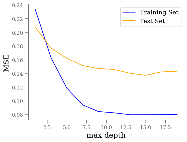
Beyond a max_depth of ~10, the MSE on the training set declines while the MSE on the test set flattens out, suggesting some amount of over-fitting.

To explore further, we will explore how general our model performance (here quantifed with MSE) is using k-fold cross-validation via sklearn. In practice, the X and y datasets are split into k “folds”, and over k iterations, the model is trained using k-1 folds as training data and the remaining fold as a test set to compute performace (i.e., MSE).

from sklearn.model_selection import cross_validate

cv = cross_validate(
    estimator=rf, 
    X=df_x, 
    y=df_y, 
    cv=5, # number of folds
    scoring='neg_mean_squared_error'
)

print(f'Cross-validated score: {cv["test_score"].mean():.3f} +/- {cv["test_score"].std():.3f}')

Cross-validated score: -0.156 +/- 0.089

The previous MSE is consistent with the cross-validated MSE, suggesting that the model is not significantly over-fitting.

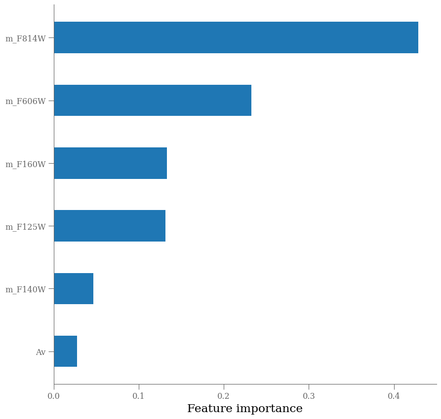
Next, we’ll observe which features are most important to the model predictions.

importances = rf.feature_importances_
argsort = np.argsort(importances)
fig = plt.figure(figsize=[10, 10])
ax = fig.add_subplot(111)
ax.barh(np.arange(len(df_x.columns)), importances[argsort], 
        align='center', 
        height=0.5, 
        tick_label=np.array(df_x.columns)[argsort])
ax.set_xlabel("Feature importance")

Text(0.5, 0, 'Feature importance')

Extratrees

from sklearn.ensemble import HistGradientBoostingRegressor


# Initialize the model
et = HistGradientBoostingRegressor()

et.fit(X_train, y_train)

HistGradientBoostingRegressor()

In a Jupyter environment, please rerun this cell to show the HTML representation or trust the notebook.
On GitHub, the HTML representation is unable to render, please try loading this page with nbviewer.org.

y_predict = et.predict(X_test)
y_predict0 = et.predict(X_train)
mse_train = mean_squared_error(y_train, y_predict0)
mse_test = mean_squared_error(y_test, y_predict)

fig, ax = plt.subplots(1, 1, figsize=(4, 4))
ax.scatter(y_test, y_predict, alpha=0.2, label=f'test mse={mse_test:0.4f}')
ax.scatter(y_train, y_predict0, alpha=0.2, label=f'train mse={mse_train:0.4f}', zorder=-1)
ax.plot(ax.get_xlim(), ax.get_xlim(), zorder=-1, color='0.5')
ax.set_aspect('equal')
ax.set_xlim(-0.1, 5)
ax.set_ylim(-0.1, 5)
ax.set_xlabel('Truth (y_test)')
ax.set_ylabel('Prediction (y_predict)')
plt.legend(loc='best')

<matplotlib.legend.Legend at 0x7f22c90eb250>

cv = cross_validate(
    estimator=et, 
    X=df_x, 
    y=df_y, 
    cv=5, # number of folds
    scoring='neg_mean_squared_error'
)

print(f'Cross-validated score: {cv["test_score"].mean():.3f} +/- {cv["test_score"].std():.3f}')

Cross-validated score: -0.154 +/- 0.088

pipe2 = Pipeline([
    ('polynomial', PolynomialFeatures(degree=3)),
    ('scaler', StandardScaler()),
    ('classifier', HistGradientBoostingRegressor())
])

pipe2.fit(X_train, y_train)

Pipeline(steps=[('polynomial', PolynomialFeatures(degree=3)),
                ('scaler', StandardScaler()),
                ('classifier', HistGradientBoostingRegressor())])

In a Jupyter environment, please rerun this cell to show the HTML representation or trust the notebook.
On GitHub, the HTML representation is unable to render, please try loading this page with nbviewer.org.

y_predict = pipe2.predict(X_test)
y_predict0 = pipe2.predict(X_train)
mse_train = mean_squared_error(y_train, y_predict0)
mse_test = mean_squared_error(y_test, y_predict)

fig, ax = plt.subplots(1, 1, figsize=(4, 4))
ax.scatter(y_test, y_predict, alpha=0.2, label=f'test mse={mse_test:0.4f}')
ax.scatter(y_train, y_predict0, alpha=0.2, label=f'train mse={mse_train:0.4f}', zorder=-1)
ax.plot(ax.get_xlim(), ax.get_xlim(), zorder=-1, color='0.5')
ax.set_aspect('equal')
ax.set_xlim(-0.1, 5)
ax.set_ylim(-0.1, 5)
ax.set_xlabel('Truth (y_test)')
ax.set_ylabel('Prediction (y_predict)')
plt.legend(loc='best')

<matplotlib.legend.Legend at 0x7f22c915ada0>

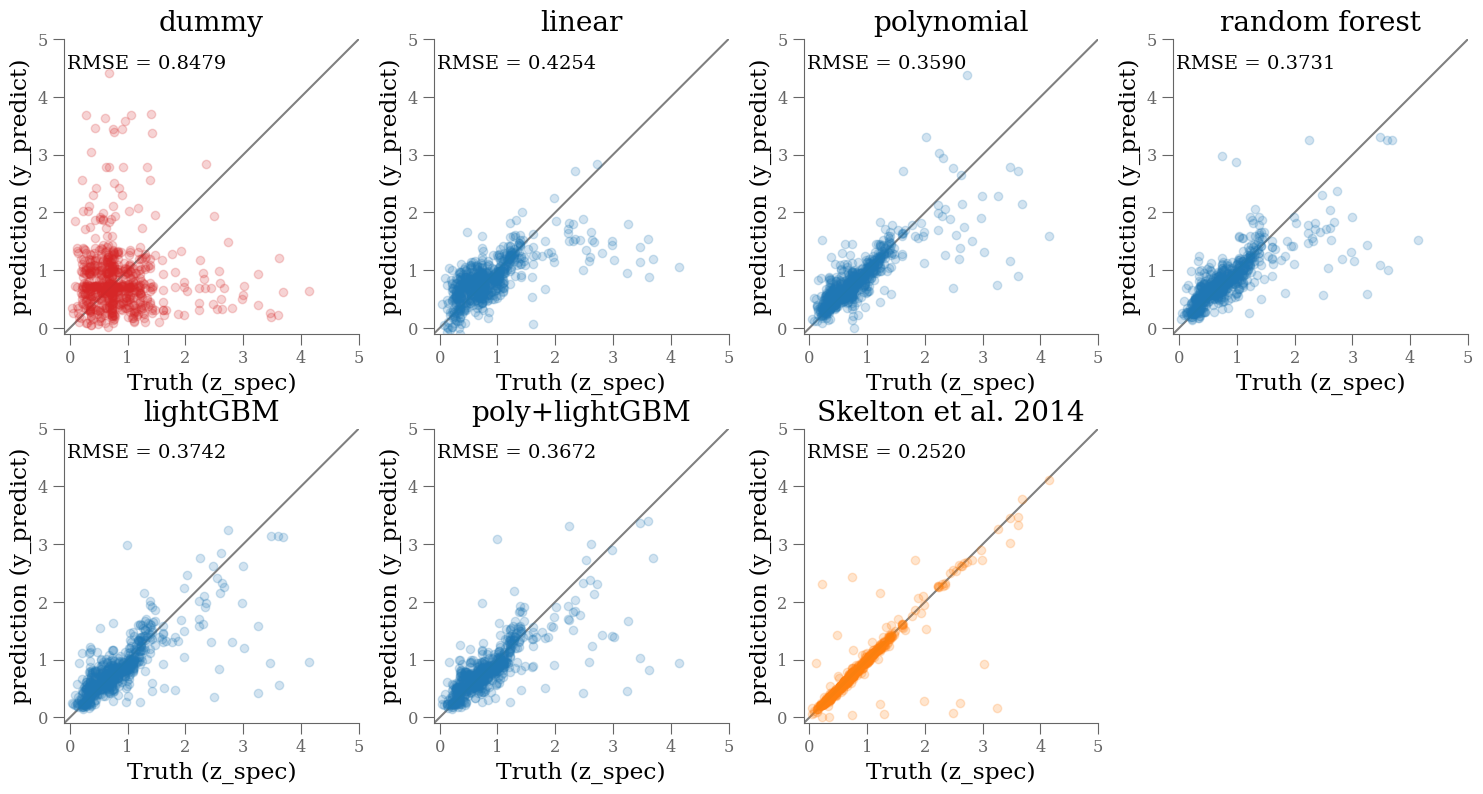
Check against each other and reference

n, bins = np.histogram(y_train, bins=256)
cdf = n.cumsum()
z_cdf = 0.5 * (bins[:-1] + bins[1])
yval = np.interp(np.random.uniform(0, 1, len(y_test)),
                 cdf / cdf[-1], bins[:-1])

y_values = [yval[:], 
            lin.predict(X_test),
            pipe.predict(X_test),
            rf.predict(X_test),
            et.predict(X_test),
            pipe2.predict(X_test),
            df_['z_peak'].loc[y_test.index]
]

names = ['dummy', 'linear', 'polynomial', 'random forest', 'lightGBM', 'poly+lightGBM', 'Skelton et al. 2014']

wrap = 4

nlines = (len(columns) + 1) // wrap +  int((len(columns) + 1) % wrap > 0)

# plt.figure(figsize=(15, nlines * 4))

fig, axes = plt.subplots(nlines, wrap, figsize=(15, 4 * nlines))

for k, (ax, yval) in enumerate(zip(np.ravel(axes), y_values)):
    color = 'C0'
    if k == len(names) - 1:
        color = 'C1'
    if k == 0:
        color='C3'
    ax.scatter(y_test, yval, alpha=0.2, color=color)
    ax.set_aspect('equal')
    ax.set_xlim(-0.1, 5)
    ax.set_ylim(-0.1, 5)
    ax.plot(ax.get_xlim(), ax.get_xlim(), zorder=-1, color='0.5')
    ax.set_xlabel('Truth (z_spec)')
    ax.set_ylabel('prediction (y_predict)')
    ax.set_title(names[k])
    mse = mean_squared_error(y_test, yval, squared=False)
    ax.text(0.01, 0.9, f'RMSE = {mse:.4f}', transform=ax.transAxes)
plt.setp(np.ravel(axes)[k+1:], visible=False)

plt.tight_layout()

Going further

• What if you include galaxy colors (e.g., F125W-F140W, F140W-F160W, F606W-F125W)? do the model results improve? Can you think of other features to include?

• Can you tune the model parameters with a grid search?

• What if you try other models from sklearn?

Neural Networks

from typing import Sequence
import torch

class linearRegressionNN(torch.nn.Module):
    def __init__(self, n_input: int, 
                 n_hidden: Sequence[int], 
                 n_output: int):
        super().__init__()
    
        self.sequence = torch.nn.Sequential()
        # add input layer
        self.sequence.add_module("input", 
                                 torch.nn.Linear(n_input, n_hidden[0]))
        # set hidden layers
        for e, (n1, n2) in enumerate(zip(n_hidden[:-1], n_hidden[1:])):
            self.sequence.add_module(f"hidden_{e:d}", 
                                     torch.nn.Linear(n1, n2))
            self.sequence.add_module(f"activation_{e:d}", 
                                     torch.nn.SELU())
        # set output layer    
        self.sequence.add_module("output",  
                                 torch.nn.Linear(n_hidden[-1], n_output))

    def forward(self, x: torch.Tensor) -> torch.Tensor:

        return self.sequence(x)

criterion = torch.nn.MSELoss()

/shared-libs/python3.10/py/lib/python3.10/site-packages/tqdm/auto.py:22: TqdmWarning: IProgress not found. Please update jupyter and ipywidgets. See https://ipywidgets.readthedocs.io/en/stable/user_install.html
  from .autonotebook import tqdm as notebook_tqdm

model = linearRegressionNN(len(features), [32] * 4, 1)
optimizer = torch.optim.RAdam(model.parameters(), lr=1e-3, weight_decay=1e-4)
criterion = torch.nn.MSELoss()
epochs = 6_000

# always be careful to normalize your data.
x_scaler = StandardScaler()
X_scaled = np.squeeze(x_scaler.fit_transform(X_train))
inputs = torch.from_numpy(X_scaled.astype('float32'))
labels = torch.from_numpy(y_train.to_numpy().astype('float32').reshape(-1, 1))
inputs_test = torch.from_numpy(x_scaler.transform(X_test).astype('float32'))
labels_test = torch.from_numpy(y_test.to_numpy().astype('float32').reshape(-1, 1))

# monitoring
loss_list = []
history = [] 

for epoch in range(epochs):
    # Clear gradient buffers because we don't want any gradient 
    # from previous epoch to carry forward, dont want to cummulate gradients
    optimizer.zero_grad()

    # get output from the model, given the inputs
    outputs = model(inputs)
    outputs_test = model(inputs_test)

    # get loss for the predicted output
    loss = criterion(outputs, labels)
    loss_test = criterion(outputs_test, labels_test)
    # get gradients w.r.t to parameters
    loss.backward()

    # update parameters
    optimizer.step()

    if epoch % 100 == 0:
        print('epoch {}, loss {:2.4g} {:2.4g}'.format(epoch, loss.item(), loss_test.item()))
    history += [[epoch, float(loss), float(loss_test)]]    
    #scheduler.step()

print(f"Epoch= {epoch},\t loss = {loss:2.4g} {loss_test:2.4g}")
print('done.')

epoch 0, loss 1.256 1.194
epoch 100, loss 0.2532 0.2278
epoch 200, loss 0.2139 0.1975
epoch 300, loss 0.2004 0.1835
epoch 400, loss 0.1863 0.1683
epoch 500, loss 0.1766 0.1581
epoch 600, loss 0.1671 0.1524
epoch 700, loss 0.1582 0.1492
epoch 800, loss 0.1512 0.148
epoch 900, loss 0.1441 0.1448
epoch 1000, loss 0.135 0.1381
epoch 1100, loss 0.1252 0.1304
epoch 1200, loss 0.1153 0.1273
epoch 1300, loss 0.1071 0.1248
epoch 1400, loss 0.09918 0.1177
epoch 1500, loss 0.09319 0.1151
epoch 1600, loss 0.08701 0.1111
epoch 1700, loss 0.08287 0.1121
epoch 1800, loss 0.07684 0.1062
epoch 1900, loss 0.0748 0.102
epoch 2000, loss 0.07119 0.1002
epoch 2100, loss 0.0688 0.09899
epoch 2200, loss 0.06734 0.09871
epoch 2300, loss 0.06555 0.09761
epoch 2400, loss 0.06401 0.09789
epoch 2500, loss 0.06564 0.09763
epoch 2600, loss 0.06504 0.1043
epoch 2700, loss 0.06077 0.09725
epoch 2800, loss 0.06038 0.09661
epoch 2900, loss 0.06069 0.09704
epoch 3000, loss 0.05867 0.09635
epoch 3100, loss 0.05673 0.09808
epoch 3200, loss 0.05559 0.09761
epoch 3300, loss 0.05544 0.0981
epoch 3400, loss 0.05458 0.09742
epoch 3500, loss 0.0554 0.09712
epoch 3600, loss 0.05304 0.09779
epoch 3700, loss 0.05986 0.1105
epoch 3800, loss 0.05138 0.09794
epoch 3900, loss 0.05086 0.09789
epoch 4000, loss 0.05482 0.09978
epoch 4100, loss 0.05071 0.09806
epoch 4200, loss 0.05018 0.09988
epoch 4300, loss 0.04906 0.09885
epoch 4400, loss 0.04861 0.09787
epoch 4500, loss 0.04919 0.1017
epoch 4600, loss 0.0478 0.09805
epoch 4700, loss 0.0476 0.101
epoch 4800, loss 0.04932 0.1013
epoch 4900, loss 0.04768 0.09877
epoch 5000, loss 0.04649 0.09809
epoch 5100, loss 0.04653 0.09777
epoch 5200, loss 0.04514 0.09801
epoch 5300, loss 0.04489 0.09818
epoch 5400, loss 0.04561 0.09733
epoch 5500, loss 0.04413 0.09794
epoch 5600, loss 0.04747 0.1043
epoch 5700, loss 0.04582 0.1024
epoch 5800, loss 0.04401 0.09853
epoch 5900, loss 0.04362 0.0974
Epoch= 5999,	 loss = 0.04279 0.09795
done.

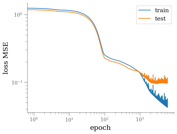
plt.loglog([e for (e, l, _) in history], 
           [float(l) for (e, l, _) in history], '-', label='train')
plt.loglog([e for (e, _, l) in history], 
           [float(l) for (e, _, l) in history], '-', label='test')
plt.legend()
plt.xlabel('epoch')
plt.ylabel('loss MSE')

Text(0, 0.5, 'loss MSE')

y_predict = model(
    torch.from_numpy(x_scaler.transform(X_test).astype('float32'))
    ).cpu().detach().numpy()  
y_predict0 = model(
    torch.from_numpy(x_scaler.transform(X_train).astype('float32'))
    ).cpu().detach().numpy()  

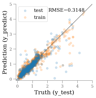
mse = mean_squared_error(y_test, y_predict, squared=False)
print(f'RMSE = {mse:.4f}')

fig, ax = plt.subplots(1, 1, figsize=(4, 4))
ax.scatter(y_test, y_predict, alpha=0.2, label='test')
ax.scatter(y_train, y_predict0, alpha=0.2, label='train', zorder=-1)
ax.plot(ax.get_xlim(), ax.get_xlim(), zorder=-1, color='0.5')
ax.set_aspect('equal')
ax.set_xlim(-0.1, 5)
ax.set_ylim(-0.1, 5)
ax.set_xlabel('Truth (y_test)')
ax.set_ylabel('Prediction (y_predict)')
plt.legend(loc='best')
ax.text(0.9, 0.9, f"RMSE={mse:0.4f}", transform=ax.transAxes, ha='right');

RMSE = 0.3148