Introduction to Deep Learning & Neural Networks

Introduction to Deep Learning & Neural Networks#

The world of data analysis and machine learning is growing rapidly. As a scientist, you may be wondering what deep learning and neural networks are all about. I provide a short introduction to these topics with an emphasis on their potential applications in the field of data analysis and astronomy.

Deep Learning refers to artificial neural networks (ANNs) that use multiple layers of neurons for more complex tasks such as pattern recognition or image classification. Deep Learning models can learn patterns from large amounts of data by adjusting connections between different layers until desired performance is achieved - making them ideal for complex problems such as computer vision or natural language processing (NLP).

Python libraries like TensorFlow, Keras, PyTorch, Theano, Jax, etc., allow scientists to easily create powerful deep learning models without having extensive knowledge on coding algorithms themselves. These libraries enable researchers and developers alike to quickly prototype new ideas using pre-existing architectures while still allowing flexibility when needed for custom implementations. These libraries may be too easy to use for research and development purposes, as often users do not need some understanding to obtain the results of their research leading to sometimes mistakes.

However, Deep learning models are not an answer to all problems, there are some downsides associated with using them: they require significant computational resources during both training and inference phases ; additionally due lackof transparency around how decisions were reached makes them difficult debug and interpret results obtained through DL models ; finally even though DL has seen tremendous progress over past few years its far away from being able to solve any problem given enough compute resources. We need take careful consideration when deciding whether DL approach should used instead traditional ML techniques available today.

All things considered, make sure familiarize yourself basics if wish stay ahead curve and do good science!

What is deep learning?#

In its essence, Deep Learning (DL) is one of many techniques collectively known as machine learning. Machine learning (ML) refers to techniques where a computer “learns” by examples. Machine learning is part of the grand scheme of automated machine decisions. People often refer machine learning as being a form of artificial intelligence (AI). AI is broad and aims at tackling problems the way humans do but to first order designates systems that learn or adapt decision rules. In computer science, a rule-based system is a system that stores and manipulate knowledge to interpret information or take decisions in a useful way. Normally, the term rule-based system only applies to systems involving human-crafted or curated rule sets. For instance in a factory, if an item is not conforming to the size or shape rule, it will be discarded.

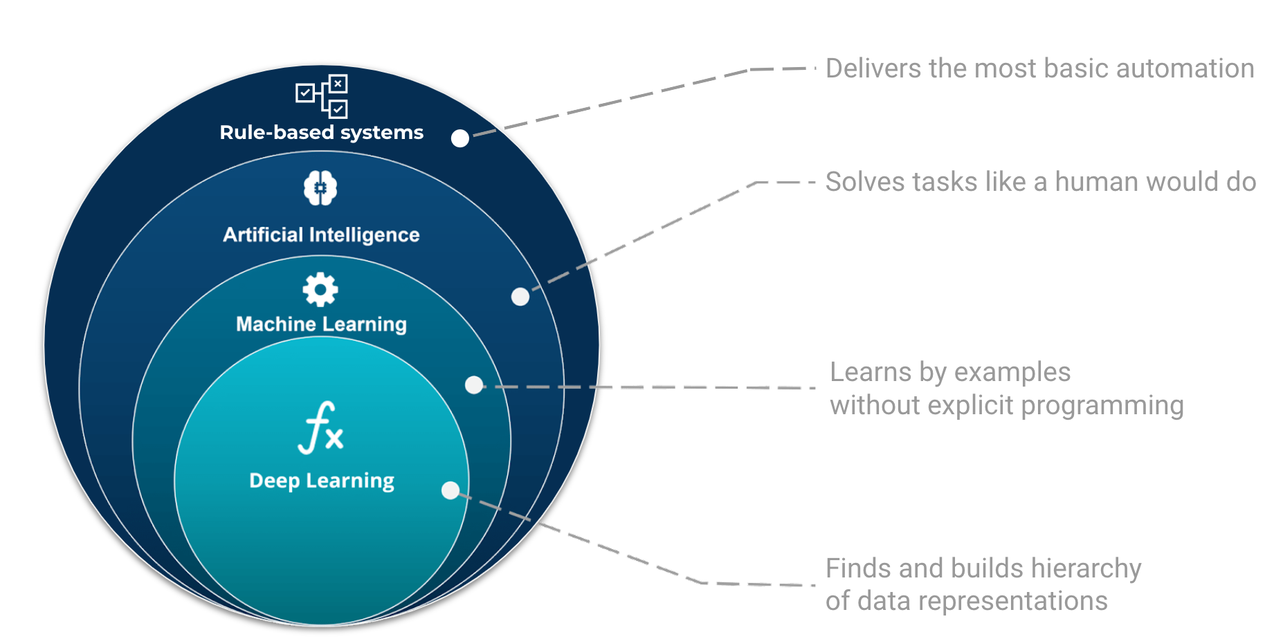
Fig. 15 The place and role of AI, ML, and Deep Learning in automated machine decisions. Image adapted from Tukijaaliwa, CC BY-SA 4.0, via Wikimedia Commons, original source#

Building blocks of neural networks#

Neurons#

A first unit of neural networks is the neuron. A neuron takes a set of inputs ($x_{1}, \ldots, x_{n}$), does a weighted sum and apply some simple function to the latter to produce one output. The following is a schematics of a neuron with three inputs.

../../_images/fcd191316349dd6c2d1856a6eba4fd75a4872f7c34316b43f5e53238795a0fe4.svg

In this example, the output corresponds to $$output = f(w_1 \cdot x_1 + w_2 \cdot x_2 + w_3 \cdot x_3)$$

$f$ is called activation function. The activation function is used to turn an unbounded input into an output that has a predictable form.

What is a Neural Network Activation Function?#

An Activation Function is a function applied on the output of a neuron and decides whether it should be “activated”. It does not have to output a binary decision. The role of the activation function is to rank the input importance in the process of prediction using simple mathematical operations.

The primary role of the Activation Function is to transform the summed weighted input from the node into an output value fed to the next network layer.

Tip

In deep learning, the Activation Function is often referred to as a Transfer Function in Artificial Neural Network.

The following figure illustrates some of the most common activation functions. These do not have to be bounded to outputs in [0, 1] intervals. Note also that activations functions could be parametric and those parameters adjusted during the training phase similarly to the weights.

../../_images/7634abde8264be8f7e464d3da17061ae72199d89090a824cd9850e8a590bbc2f.png

How to choose the right Activation Function?#

Activation functions could vary within a network. But any choice need to match activation functions to the outputs based on the type of problem to solve.

As a rule of thumb, ReLU is a good activation function to start with in most problems. But it won’t always provide the best performance. But the following list gives some guidelines:

ReLU activation function should only be for the hidden layers.
Sigmoid and Tanh functions are not for in hidden layers as they make the model more susceptible to training issues(vanishing gradients).
Swish function is recommended in neural networks with 40 hidden layers and more.

The following provides some recommendation for the output layer based on the type of prediction problem that you are solving:

Regression: Linear Activation Functions
Binary Classification: Sigmoid/Tanh Activation Function
Multiclass Classification: Softmax
Multilabel Classification: Sigmoid

The activation function in hidden layers is typically dependent on the type of neural network architecture. As a first try, we will use the following activation function:

Convolutional Neural Network (CNN): ReLU (or SeLU etc)
Recurrent Neural Network: Tanh and/or Sigmoid.

Note

All hidden layers usually use the same activation function. However, the output layer can typically use a different activation function from the hidden layers. The choice depends on the goal or type of prediction made by the model.

Simple Example#

Let’s assume we have a three-input neuron with a ReLU activation function and the following weights:

\[ w=[0, 1, 4]. \]

What will be the output to an input vector $x = [2, 3, 1]$ and $x^\prime = [1, -3, 0]$?

\[\begin{split} \begin{aligned} y &= f(w \cdot x) \\ &= f([0, 1, 4] \cdot [2, 3, 1]) \\ &= f(7) \\ &= 7 \end{aligned} \end{split}\]

\[\begin{split} \begin{aligned} y^\prime &= f(w \cdot x^\prime) \\ &= f([0, 1, 4] \cdot [1, -3, 0]) \\ &= f(-3) \\ &= 0 \end{aligned} \end{split}\]

Important

This process of passing inputs forward to get an output is known as feedforward.

What value do we obtain with a sigmoid function? What about other activation functions?

import pandas as pd
values = {name: [np.round(fn(7), 3), np.round(fn(-3), 3)] for name, fn in zip(labels, fns)}
values['preact'] = [7, -1]
pd.DataFrame.from_dict(values).set_index('preact')

	linear	sigmoid	tanh	ReLU	leaky_ReLU	ELU	swich	SELU	GELU
preact
7	7	0.999	1.000	7	7.0	7.00	6.994	7.350	7.000
-1	-3	0.047	-0.995	0	-0.3	-0.95	-0.142	-1.666	-0.004

Example with coding a Neuron#

Let’s manually implement a neuron using NumPy.

first define a ReLU activation function as $f(x) = \max(0, x)$
define a class Neuron which takes a vector of weights at initialization
define the Neuron.forward method which takes a vector of inputs and returns the output of the neuron
evaluate the code with the previous values.

Tip

class Neuron:
  def __init__(self, weights: np.ndarray, activation: Callable):
    pass

  def forward(self, inputs: np.ndarray) -> np.ndarray:
    pass

[2, 3, 1] -->  7
[1, -3, 0] -->  0

Combining Neurons to create a network#

With a single neuron, we can create a scaled weighted sum operator. With a linear activation function, a single neuron corresponds to a linear regression model.

But with many connected neurons we can generate more complex operations.

The following example network has 3 inputs, a single hidden layer with 3 neurons an one output layer with 1 neuron.

A hidden layer corresponds to any layer between the input (first) layer and output (last) layer. There can be many hidden layers (deep network)

../../_images/440ab20f7db6b184562fcc207637bc1381eebedb56a90b25942cf2a59551881f.svg

A neural network can have any number of layers with any number of neurons in those layers. The basic idea stays the same: feed the input(s) forward through the neurons in the network to get the output(s) at the end. For simplicity, we’ll keep using the network pictured above for the rest of this post.

We will skip the pen and paper calculations and implement this network in Python.

class NeuralNetwork:
    
    def __init__(self, 
        input_size: int, 
        hidden_size: int, 
        output_size: int, 
        weights: List[float] = None, 
        activation: Callable = sigmoid):
        pass

    def forward(self, X):
        pass

model = NeuralNetwork(3, 3, 1, activation=sigmoid)
model.forward([2, 3, 1])

Tip

This implementation is freeform. You can use the previous Neuron class, make a Dense layer or work with arrays of weights.

np.random.seed(42)
model = NeuralNetwork(3, [3], 1, activation=sigmoid)
model.forward([2, 3, 1])

array([0.45125419])

The weights are initialized at random and therefore without imposing the weights and doing the calculations by hand, it will be difficult to verify the model. Let’s train our model instead.

Training a Neural Network#

Let’s use the common iris dataset, a multivariate data set used and made famous by the British statistician and biologist Ronald Fisher in his 1936 paper.

The data set consists of 50 samples from each of three species of Iris (setosa, virginica, and versicolor) and four measurements from each sample: the length and the width of the sepals and petals, in centimeters.

from sklearn.datasets import load_iris
iris = load_iris()
iris.keys()

dict_keys(['data', 'target', 'frame', 'target_names', 'DESCR', 'feature_names', 'filename', 'data_module'])

Using this dataset, let’s create a neural network model to predict the species given the measurements.

np.random.seed(42)
X = iris['data']
y = iris['target']

model = NeuralNetwork(X.shape[-1], [3], 1, activation=sigmoid)
model.forward(X[0])

array([0.30257269])

The Loss function#

Before we train our network, we first need to define a performance metric which the training procedure will optimize.

For simplicity here, we will use the Mean Squared Error (MSE) as the loss function:

\[ MSE = \frac{1}{N} \sum_{i=1}^N (y_i - \hat{y}_i)^2, \]

where $N$ is the number of samples, $y_i$ is the true label, and $\hat{y}_i$ the output prediction of the network. The better our predictions, the lower MSE value, i.e. lower loss.

Important

the training procedure minimizes the loss function given a training set

def mse(y_true: np.array, y_pred: np.array) -> float:
    return np.mean((y_true - y_pred) ** 2)

yhat = np.array([model.forward(xk) for xk in X])
print("MSE loss (t=0) = ", mse(y, yhat))

MSE loss (t=0) =  1.2194368145413368

Now we have to optimize this function, i.e. the loss of the neural network. We can adjust the network’s weights to change the predictions.

Optimization and backpropagation#

Warning

This part is a bit mathematical.

The loss function $L$ is function of all the weights $W$ and we want to minimize $L$ w.r.t $W$.

Let’s look at optimizing a single weight $w_{11}$ corresponding to the connection of the $x_{1}$ with the first neuron in the hidden layer $h_1$. The derivative of $L$ w.r.t. $w_{11}$ is

\[\begin{split}\begin{align} \frac{\partial L}{\partial w_{11}} &= \frac{\partial L}{\partial \hat{y}} \cdot \frac{\partial \hat{y}}{\partial w_{11}} \\ \frac{\partial L}{\partial \hat{y}} &= -2 (y - \hat{y}) \end{align}\end{split}\]

The other term is a bit more complicated. But since $w_{11}$ is between $x_1$ and $h_1$:

\[\begin{split}\begin{align} \frac{\partial \hat{y}}{\partial w_{11}} &= \frac{\partial \hat{y}}{\partial h_1} \cdot \frac{\partial h_1}{\partial w_{11}} \\ \frac{\partial \hat{y}}{\partial h_1} &= w_{21} \cdot f^\prime(w_{21} h_1 + w_{22} h_2 + w_{23} h_3)\\ \frac{\partial h_1}{\partial w_{11}} &= x_1 \cdot f^\prime(w_{11} x_1 + w_{12} x_2 + w_{13} x_3) \end{align}\end{split}\]

Finally, most activation functions $f$ have relatively simple derivative $f^\prime$. For instance, the sigmoid function has a simple derivative

\[\begin{split}\begin{align} f(x) &= \frac{1}{1 + e^{-x}} \\ f^\prime(x) &= \frac{e^{-x}}{(1 + e^{-x})^2} = f(x) \cdot (1 - f(x)) \end{align}\end{split}\]

We managed to express all the necessary terms in the derivative of $L$ w.r.t. $w_{11}$:

\[\begin{align} \frac{\partial L}{\partial w_{11}} &= \frac{\partial L}{\partial \hat{y}} \cdot \frac{\partial \hat{y}}{\partial h_{1}} \cdot \frac{\partial {h_1}}{\partial w_{11}} \end{align}\]

This system of calculating partial derivatives by working backwards is known as backpropagation. Backpropagation is the process of finding the derivative of the loss function w.r.t. all the weights $W$.

Training through Stochastic Gradient Descent#

The final step of our model is to minimize the loss function w.r.t. all the weights using our training data.

A traditional approach uses an optimization algorithm essentially based on stochastic gradient descent (SGD). It is a variant of Gradient Descent (GD) but it uses only a random subset of the training data (also known as a mini-batch) rather than the entire training data set to calculate the gradient of the loss function. This random selection of data provides faster and more frequent updates to the model parameters, making it more efficient than GD when the data set is large. SGD repeats this process for a fixed number of iterations or until the convergence of the loss function.

The learning rate $\eta$ is an hyperparameter that controls the step size at each iteration, e.g.:

\[ w_1 \leftarrow w_{11} - \eta \frac{\partial L}{\partial w_{11}} \]

If we do this for every weight in the network, the loss will slowly decrease and our network will improve.

The SGD training process will look like this:

Choose one random sample/subset from our dataset.
Calculate all the partial derivatives of loss with respect to weights
Update the weights by subtracting the learning rate times the partial derivatives. and repeat until convergence.

To avoid having to code everything in the following we use sklearn.neural_network.MLPClassifier which implements an SGD optimizer (as well as others).

from sklearn.neural_network import MLPClassifier

model = MLPClassifier(solver='sgd',
    alpha=1e-5, hidden_layer_sizes=(3, 3),
    random_state=1, max_iter=10_000)
model.fit(X, y)

yhat = model.predict(X)
print("Final loss: ", mse(y, yhat))

Final loss:  0.02

We can also visualize the loss values as function of the training iterations, aka epoch

plt.plot(model.loss_curve_)
plt.xlabel('Epochs')
plt.ylabel('Loss (MSE)')

Text(0, 0.5, 'Loss (MSE)')

../../_images/98f0a9acfcb4f1a667dec0cc94e0b99e4ab6c633d4c518dd26b3206f8b5cb919.png

plt.figure(figsize=(10, 5))
plt.subplot(1, 2, 1)
plt.scatter(X[:, 0], X[:, 1], c=y, cmap='jet')
plt.xlabel('$x_0$')
plt.ylabel('$x_1$')
plt.title('training data')
plt.subplot(1, 2, 2)
yhat = model.predict(X)
plt.scatter(X[:, 0], X[:, 1], c=yhat, cmap='jet')
plt.xlabel('$x_0$')
plt.ylabel('$x_1$')
plt.title('predictions')
plt.tight_layout()

../../_images/f8333244d4ed6493f9c31608af0a4268a7da8be4691432a8eb6a6cdde0981e03.png

Why are deep neural networks hard to train?#

Training NNs may sometimes lead to catastrophic failures (e.g., wrong activation function, forgetting to normalize the input data). There are two major challenges you might encounter when training your deep networks.

Vanishing Gradients#

Like the sigmoid function, certain activation functions compress an infinite interval into [0, 1]. Hence, their derivative becomes small. For shallow networks with only a few layers that use these activations, this isn’t a big problem. But, when networks contain more layers, the product of those gradients becomes too small for training to work effectively.

Exploding Gradients#

Exploding gradients occurs when significant error gradients accumulate and result in very large updates to neural network model weights during training with SGD based optimizers. With these exploding gradients, you can obtain unstable networks and the learning cannot be completed.

The values of the weights can also become so large as to overflow.

Key vocabulary

Artificial Neural Network (ANN): A computational system inspired by the way biological neural networks in the human brain process information.
Neuron: A building block of ANN. It is responsible for accepting input data, performing calculations, and producing output.
Deep Neural Network: An ANN with many layers placed between the input layer and the output layer.
Input data: Information or data provided to the neurons.
Weights: The strength of the connection between two neurons. Weights determine what impact the input will have on the output.
Bias: An additional parameter used along with the sum of the product of weights and inputs to produce an output.
Activation Function: Determines the output of a neural network.
Feed forward (forward propagation): The process of feeding the input data to the neurons.
Back propagation (back propagation): The process of adjusting the weights and biases of the neurons through the gradient of the loss function.

Advantages & Disadvantages of Neural Networks#

Advantages#

Fault tolerance: even if a few neurons are not “working” properly, that would not prevent the neural networks from generating outputs.
Real-time Operations: neural networks can learn synchronously and easily adapt to their changing environments.
Adaptive Learning: neural networks can learn how to work on different tasks, or sub-tasks with proper training.
Parallel processing capacity: neural networks can perform multiple tasks simultaneously.

Disadvantages#

Unexplained behavior of the network: neural networks provide a solution to a problem but rarely a why and how it made the decisions it made. Understanding the behavior of a model represents additional tasks to the architect (i.e., the user).
Determination of appropriate network structure: there is no generic rule (or rule of thumb) to design a neural network architecture. A proper network structure is achieved by trying the best network, in a trial and error approach. It is a process that involves refinement.
Hardware dependence: To be efficient in computational speed (training or evaluation), neural networks require (or are highly dependent on) processors (CPU, GPU, TPU) with adequate processing capacity.

What sort of problems can Deep Learning not solve?#

DL is not always capable to solve problems. It will not work in

any case where only a small amount of training data is available,
tasks requiring an explanation of how the answer was arrived at (interpretability not guaranteed),
Classifying things which are nothing like their training data (not good at genaralization).

What sort of problems can Deep Learning solve but should not be used for?#

Deep Learning needs a lot of computational power, it often relies on specialised hardware like graphical processing units (GPUs). Many computational problems can be solved using less intensive techniques, but could still technically be solved with Deep Learning. It is tempting to use the fashion techniques to solve old problems, but we should remain critical.

Deep learning can technically solve the following but it would probably be a wasteful way to do it:

Logic operations, such as sums, averages, ranges etc.
Modelling well defined systems, where the equations governing them are known and understood.
Basic computer vision tasks such as edge detection, decreasing colour depth or blurring an image.

Deep Learning Libraries#

There are many software libraries available for Deep Learning. Python includes:

TensorFlow#

TensorFlow was developed by Google and is one of the older Deep Learning libraries, ported across many languages since it was first released to the public in 2015. It is very versatile and capable of much more than Deep Learning but as a result it often takes a lot more lines of code to write Deep Learning operations in TensorFlow than in other libraries. It offers (almost) seamless integration with GPU accelerators and Google’s own TPU (Tensor Processing Unit) chips that are built specially for machine learning.

PyTorch#

PyTorch was developed by Facebook in 2016 and it is a popular choice for Deep Learning applications. It was developed for Python from the start and feels a lot more “pythonic” than TensorFlow. Like TensorFlow it was designed to do more than just Deep Learning and offers some very low level interfaces. PyTorch Lightning offers a higher level interface to PyTorch to set up experiments. Like TensorFlow it is also very easy to integrate PyTorch with a GPU.

Keras#

Keras is designed to be easy to use and usually requires fewer lines of code than other libraries. We have chosen it for this workshop for that reason. Keras can actually work on top of TensorFlow (and several other libraries), hiding away the complexities of TensorFlow while still allowing you to make use of their features.

The performance of Keras is sometimes not as good as other libraries and if you are going to move on to create very large networks using very large datasets then you might want to consider one of the other libraries. But for many applications the performance difference will not be enough to worry about and the time you will save with simpler code will exceed what you will save by having the code run a little faster.

Jax + Flax#

Jax is a Python library developed by Google for high-performance numerical computing and machine learning. It provides an interface that is similar to NumPy but that can run on GPUs and TPUs transparently for the users offering significantly improved performance. JAX includes automatic differentiation, which makes it easy to train machine learning models using techniques like stochastic gradient descent.

Flax is a neural network library that is built on top of JAX and is designed for flexibility . It provides a high-level API for defining and training neural networks and has built-in support for advanced training techniques like mixed precision and gradient checkpointing.

Which library should I use/learn?#

There are no standard answer to which library should I use or learn, even when having a specific problem.

TensorFlow and PyTorch are currently the most widely used deep learning libraries, while JAX is growing in popularity due to its efficient GPU and TPU acceleration, automatic differentiation, and high flexibility.

It is important to note that Google currently slows down the development of Tensorflow in favor of JAX. But Tensorflow remains the most common library for insdustry applications. It provides many services and pre-trained models.

Jax is the new kid in the playground. Its development is extremely fast, and it gets a lot of traction in the scientific community.

Exercise: Logical XOR network#

In this exercise, you will implement a simple XOR network, i.e. implement a network that exactly matches the behavior of a simple logical XOR operator.

For this exercise, the network needs at least one hidden layer to solve the problem.

Logical XOR#

XOR stands for “exclusive or”. The output of the XOR function has only a true value if the two inputs are different. If the two inputs are identical, the XOR function returns a false value. The following table shows the inputs and outputs of the XOR function.

%matplotlib inline
import pylab as plt
import numpy as np

# x1, x2, y
xor_data = np.array([[0, 0, 0],
                     [1, 0, 1],
                     [0, 1, 1],
                     [1, 1, 0]])
or_data = np.array([[0, 0, 0],
                    [1, 0, 1],
                    [0, 1, 1],
                    [1, 1, 1]])
and_data = np.array([[0, 0, 0],
                     [1, 0, 0],
                     [0, 1, 0],
                     [1, 1, 1]])

The following figure illustrates the logical operations OR, AND, and XOR. In contrast to OR and AND problems, the XOR one cannot be linearly separated by a single boundaryline. To solve this problem, we will need two boundary lines, hence requires at least one hidden layer in our neural network.

../../_images/531a5e763aee50844fb9b909e94c64c27b5c7b844f6eaa3c7368f1f24d15a1d0.png

The next step is to define a Neural Network that is able to solve the XOR problem. With the correct choice of functions and weight parameters, a Neural Network with one hidden layer is able to solve the XOR problem. Because we have logical operations, a threshold activation function should be sufficient.

../../_images/6f4674816e1e53d870846fd43586f325dbc19d93506e6253302a52f631a6dc88.svg

from sklearn.neural_network import MLPClassifier, MLPRegressor
import numpy as np

np.random.seed(0)

model = MLPClassifier(
                activation='logistic',
                max_iter=20_000,
                hidden_layer_sizes=(2,),
                solver='lbfgs',
                )

X = xor_data[:, :2]
y = xor_data[:, 2]
model.fit(X, y)

X_, Y_ = np.meshgrid(np.linspace(0, 1, 200), np.linspace(0, 1, 200))
Z = model.predict(np.c_[X_.ravel(), Y_.ravel()])

ax = plt.subplot(111, aspect='equal')
plot_data(xor_data, ax)
Z = Z.reshape(X_.shape)
plt.pcolormesh(X_, Y_, Z, cmap=plt.cm.Paired_r)
plt.xlim(-0.04, 1.04)
plt.ylim(-0.04, 1.04);

../../_images/f421fd274f4fa335d47e201042ac47dfc20e12851fce9fd5a4d7ce98758319d3.png

Main architectures of neural networkds#

The deep learning field is in constant evolution. Every now and then, we find new neural network architectures in various applications. Knowing the main abbreviations (e.g., DCIGN, BiLSTM, DCGAN, etc) can be a bit overwhelming but remains important.

Fjodor van Veen provided us with a nice cheat sheet containing many of those unique architectures. Most of these are neural networks, some are completely different beasts.

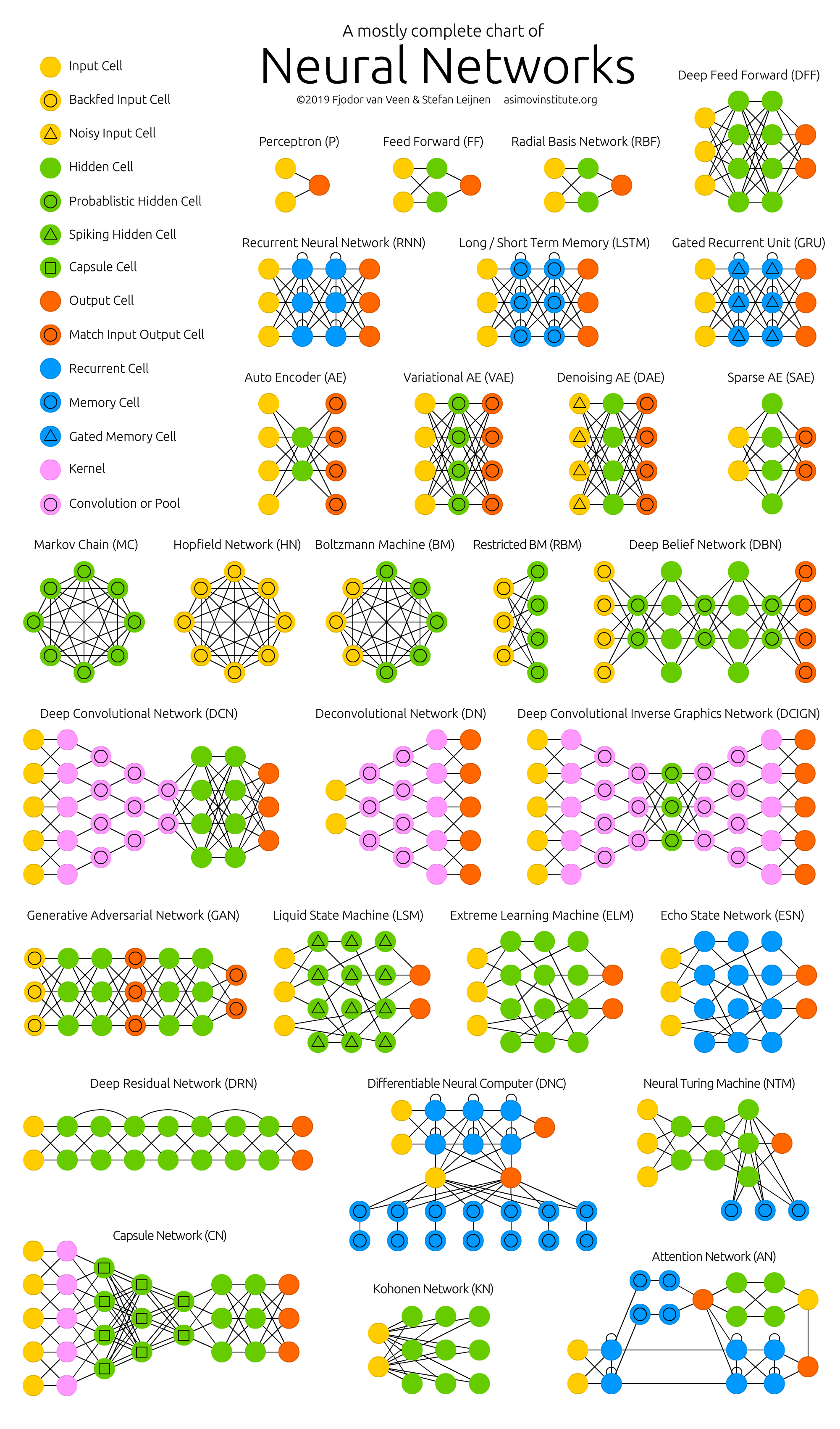
Fig. 16 The Neural Network Zoo. Credit: Van Veen, F. & Leijnen, S. (2019). The Neural Network Zoo#