Optimizing Scientific Python codes

Optimizing Scientific Python codes#

This chapter is about optimizing Python codes. Optimization is a very broad topic, from the choice of the algorithm, the hardware to the execution speed and memory footprint. Sometimes the choice of the programming language could also have a significant impact on the performance.

The primary goal of optimizing scientific codes is to make the project runs within contraints (memory limits, cpu limits, project deadline).But it is essenial before any optimization that the scientific code must be error free and packaged with some unit tests. So we will start with a section on advanced debugging.

Advanced debugging#

The best way to debug any code is to avoid bugs in the first place. This is why we have dedicated the next section to defensive programming, which aims at anticipating bugs. But even with the best practices, bugs can still happen.

The primary mechanism of debugging a code is to stop the execution of your application at particular points to inspect the state of the variables, and execute codes step by step.

Although a simple and common method is to print the value of variables at different points of the code, it is also very time consuming and not very efficient. Using appropriate tools will avoid littering your code with print statements.

../../_images/e9894be06f4b05c60613d51be7ec0c09f4127b238ed8b716bc218b26cfd8712c.png

`pdb`, the Python debugger#

`pdb`` is the standard Python debugger. It is a command-line based debugger, which opens an interactive shell, in which one can interact with the code. It allows to examine and change value of variables, execute code line by line, set up breakpoints, examine calls stack, etc.

To run a python code in debugging mode you need to run

python –m pdb script.py

To set a breakpoint at a specific line, you need to set a import pdb; pdb.set_trace() line in your code:

# some code here
# the debugger starts here
import pdb;		pdb.set_trace()
# rest of the code

Note

It is the only tolerated way to use import in the middle of a code and to have multiple instructions on the same line.

You can also use the pdb module directly in an IPython shell with the magic commands %pdb and %debug. The first one will automatically start the debugger when an exception is raised (preventive), and the second one will start the debugger at the current state, i.e. post-mortem.

The following is an example of a debugging session with pdb:

from IPython.core import debugger
debug = debugger.Pdb().set_trace


def example_function():
    import pdb; pdb.set_trace()
    filename = "tmp.py"
    print(f'path = {filename}')
    debug()

def example_function2():
    example_function()
    return 1

example_function2()

This code should result in the following output:

> /tmp/ipykernel_24227/197668726.py(7)example_function()
      5 def example_function():
      6     import pdb; pdb.set_trace()
----> 7     filename = "tmp.py"
      8     print(f'path = {filename}')
      9     debug()

Navigating the Code#

Once the debugger is started, you can navigate through your code using various commands:

l(ist): Lists 11 lines surrounding the current line.
n(ext): Executes the current line.
s(tep): Steps into functions called at the current line.
r(eturn): Executes until the current function’s return is encountered
c(ontinue): Continues execution, only stopping when a breakpoint is encountered
u(p): Moves the current frame count (default one) levels up in the stack trace (to an older frame)
d(own): Moves the current frame count (default one) levels down in the stack trace (to a newer frame)

Viewing and Changing Data#

You can also view and change data in your program:

p <expression>: Prints the value of the expression
pp <expression>: Pretty prints the value of the expression
! <statement>: Executes the (one-line) statement in the context of the current stack frame

Getting Help and Exiting#

h(elp): Shows a list of available commands. You can also show help for a specific command or topic with h
q(uit): Quits the debugger and exits

Remember, pdb is a powerful tool for debugging your Python code. It allows you to step through your code, inspect data, and understand how your code is executing, which can be especially useful when trying to track down complex bugs.

IPython `%xmode`#

The %xmode command is a magic function in IPython that allows you to control the amount of information Python reports when an exception is raised. It takes a single argument, the mode, and there are three possibilities: Plain, Context, and Verbose. The default is Context, which gives output showing the context of each step that led to the error. Plain is more compact and gives less information, while Verbose adds extra information, including the arguments to any functions that are called.

The Verbose mode can be useful when trying to debug complex code, as it provides more detailed information about the error.

def raise_error(*args, **kwargs):
    raise ValueError('This is an error')

%xmode Verbose
raise_error("Some arguments")

Exception reporting mode: Verbose

---------------------------------------------------------------------------
ValueError                                Traceback (most recent call last)
Cell In[3], line 2
      1 get_ipython().run_line_magic('xmode', 'Verbose')
----> 2 raise_error("Some arguments")

Cell In[2], line 2, in raise_error(*args=('Some arguments',), **kwargs={})
      1 def raise_error(*args, **kwargs):
----> 2     raise ValueError('This is an error')

ValueError: This is an error

Defensive programming#

Defensive programming is a programming style that aims to ensure the continuing function of a piece of code against unexpected usage. The idea behind defensive programming is to assume that errors are going to arise and write code to detect them when they do. The most common way to do this is to add assertions to the code so that it checks itself as it runs. An assertion is simply a statement that something must be true at a certain point in a program, that the variable is a float or an array for instance.

Defensive programming techniques are used especially when a piece of software could be misused mischievously or inadvertently to catastrophic effect. Defensive programming advises the programmer to improve their code keeping in mind that many things can go wrong. Preventive measures should be taken against undesirable situations that may be encountered during development, such as errors in unit, range, number of decimal places, returning None values, and choosing the right algorithm and data structure. Defensive programming can help minimize risks and make programs more reliable.

Unit tests in scientific computing#

I will not cover unit testing in details but only briefly give some reminders from chapter 3.

Unit testing is a method for testing software that looks at the smallest testable pieces of code, aka units, which execution is tested for correct behavior. In Python, unit tests are written using a testing framework such as unittest, doctest, or PyTest.

Important

unittest has been deprecated.

Unit testing is useful because it helps you catch bugs early in the development process, ensures that your code behaves as expected, and makes it easier to maintain and refactor your code. It is an essential piece during the optimization process, as it allows you to check that the code still behaves as expected after any modification.

../../_images/adcf15db170c9881741a5fd8feb5397af3ed7eadd574ecc81c16ea0778ec8d6d.svg

The basics#

It is not always clear what to test and how to properly test it. But often the most difficult part is to get started. At first it could seem cumbersome: the code obviously returns the expected answer, the test units are longer than the actual code, partial duplication, etc. But it is a good practice to write tests as you write your code. It will save you a lot of time in the long run.

I will not cover unit testing in details but only briefly give some reminders.

A good test should have several characteristics:

Isolation: Each test should be independent and able to run alone as well as part of a test suite
Thoroughness: The test should cover as much of the codebase as possible, including all possible edge cases
Repeatability: A test should produce the same results each time it is run, regardless of the order in which tests are executed
Readability: The test should be well-documented and easy to understand, so that other developers can understand what is being tested and why
Consistency: The test should consistently pass or fail, not intermittently.

When it comes to scientific code, there are some additional considerations:

Accuracy: Scientific code often involves complex calculations, so it’s crucial to test that these calculations are performed accurately
Reproducibility: Given the same input, the code should always produce the same output
Performance: Scientific code often deals with large datasets, so it’s important to test the code’s performance to ensure it can handle the data efficiently

In addition to these, it’s also recommended to follow best practices such as planning and designing your tests before writing code, using a version control system to track and manage changes, and regularly reviewing and documenting your code and tests

A good test is divided in three parts:#

Put your system in the right state for testing
- Create objects, initialize parameters, define constants…
- Define the expected result of the test
Execute the feature that you are testing
- Typically one or two lines of code
Compare outcomes with the expected ones
- Set of assertions regarding the new state of your system

Tips#

Test simple but general cases
- Take a realistic scenario for your code; try to reduce it to a simple example
Test special cases and boundary conditions
- Code often breaks because of empty lists, None, NaN, 0.0, duplicated elements, non-existing file, and what not…

Numerical traps to avoid#

Use deterministic test cases when possible
- set a seed for any randomness
For most numerical algorithm, tests cover only oversimplified situations; sometimes it is impossible
“fuzz testing”, i.e. generated random input is mostly used to stress-test error handling, memory leaks, safety, etc

Testing learning algorithm#

Learning algorithms can get stuck in local optima. The solution for general cases might not be known (e.g., unsupervised learning)
Turn your validation cases into tests (with a fixed random seed)
Stability tests:
- Start from final solution; verify that the algorithm stays there
- Start from solution and add noise to the parameters; verify that the algorithm converges back
Generate mock data from the model with known parameters
- E.g., linear regression: generate data as y = a*x + b + noise for random a, b, and x, and test# Unit tests in scientific computing

Good practice: Test-driven development (TDD)#

TDD = write your tests before your code
- Choose what is the next feature you’d like to implement
- Write a test for that feature
- Write the simplest code that will make the test pass

def construct_stellar_binary_system(
    primary: Star, 
    other: Star, 
    separation_pc: float) -> BinaryStar:
    """ combine two stars into a binary system """
    pass

def test_construct_stellar_binary_system():
    """ testing binary creation"""
    age_myr = 100
    mass_msun = 1.2
    separation_pc = 5
    primary = Star(age=age_myr, mass=mass_msun)
    secondary = Star(age=age_myr, mass=mass_msun)
    binary = construct_stellar_binary_system(primary, secondary, separation_pc)
    assert(binary_center_of_mass = separation_pc / (1 + mass_msun/mass_msun)

Pros
- Forces you to think about the design of your code before writing it. How would you like to interact with it? Functionality oriented
- The result is a code, with functions that can be tested individually.
- If the results are bad, you will always write tests to find a bug. Would you if it works fine?
Cons
- The tests may be difficult to write, especially beyond the level of unit testing.
- In the beginning, it may slow down development, but in the long run, it actually speeds up development.
- The whole team needs to buy into Unit testing for it to work well.
- can be tiresome, but it pays off big time in the end.
- Early stage refactoring requires refactoring test classes as well.

Important

Just remember, code quality is not just testing: “Trying to improve the quality of software by doing more testing is like trying to lose weight by weighing yourself more often” (Steve McConnell, Code Complete)

Optimization and Profiling#

Optimization is the process of modifying a system to make some features of it work more efficiently or use fewer resources. Who has not be faced with the issue of “Python” or “insert language name here” is slower than C? Often codes could be slow, but not prohibitively so. In scientific Python applications, This comparison is not straightforward because codes often call C/Fortran libraries (e.g. GSL, BLAS, LAPACK, etc.) without being explicitly aware of it. (e.g. Numpy, Scipy, Pandas, etc.).

Most importantly as I like to say, it is “better to have a slow working code than being fast to spill garbage”. As a reminder, the first step to optimize a code is to make sure that it giving correct outputs. Never rush into optimizations because it could easiily become be a rabbit hole.

What is the strategy to optimize codes?#

Firstly, let’s clearify that optimizing means updating the source code, not changing the algorithm or where the it runs.

Usually, a small percentage of your code takes up most of the execution time or the memory. The strategy is to identify the slowest parts of your code using a profiler and focus on exclusively optimizing these parts. As any change of the code could introduce bugs, it is important to have a good test suite to make sure that the code still works as expected. Finally, it is good to stop the optmization as soon as you deem it good enough given your project’s constraints.

Note

With Python 3.12, you can expect significant performance improvements, enhanced error reporting, and a more streamlined development experience. But caution to upgrade to Python 3.12, that some core scientific libraries are not ready!

I give below my opinion on the priority of optimization strategies:

Vectorize code (e.g. using Numpy)
Use a specific optimization toolkits (e.g., numexpr, numba, jax)
Check if compiler change could make sense (e.g., Intel’s MKL optimized libraries)
Use Cython to create compiled functions
Change approach
approximate calculations

(Again: we do not touch on parallelization of change of hardware here)

Some simple examples#

Using timeit#

The timeit module allows you to time small bits of Python code. It has both a Command-Line Interface (CLI) and a callable one. The CLI is convenient for quick tests. The callable one is convenient for repeated tests inside a program.

Precise timing of a function/expression
Test different versions of a small amount of code, often used in interactive Python shell
In IPython/Jupyter kernel, you can use the %timeit magic command.

def f(x):
    return x**2
def g(x):
    return x**4
def h(x):
    return x**8

import timeit
time_in_sec = timeit.timeit('[func(42) for func in (f,g,h)]', globals=globals(), number=1000) / 1000
print(f'{time_in_sec * 1e6: 0.3f} µs loop per 1000 run')

 1.270 µs loop per 1000 run

%timeit [func(42) for func in (f,g,h)]

1.28 µs ± 12.6 ns per loop (mean ± std. dev. of 7 runs, 1,000,000 loops each)

Note

When operations are fast, timeit automatically does a large number of repetitions. For slower commands, timeit will automatically adjust and perform fewer repetitions.

Sadly, timeit does not have convenient calls for multiple tests at once.

import timeit

subStrings=['Sun', 'Mon', 'Tue',
            'Wed', 'Thu', 'Fri',
            'Sat']

def simpleString(subStrings):
    finalString = ''
    for part in subStrings:
        finalString += part
    return finalString

def formatString(subStrings):
    finalString = "%s%s%s%s%s%s%s" % (subStrings[0], subStrings[1],
    subStrings[2], subStrings[3],
    subStrings[4], subStrings[5],
    subStrings[6])
    return finalString

def joinString(subStrings):
    return ''.join(subStrings)

print('joinString() Time   : ' + str(timeit.timeit('joinString(subStrings)', setup='from __main__ import joinString, subStrings')))
print('formatString() Time : '+ str(timeit.timeit('formatString(subStrings)', setup='from __main__ import formatString, subStrings')))
print('simpleString() Time : ' + str(timeit.timeit('simpleString(subStrings)', setup='from __main__ import simpleString, subStrings')))

joinString() Time   : 0.14162441899998157

formatString() Time : 0.375528796000026

simpleString() Time : 0.3777920879999783

The above example demonstrates that the join method is a bit more efficient than the others.

See more examples in the timeit documentation

Note

The above timeit example also accounts for the time spent in the setup statement, which is not always what you want.

Profiling code, cProfile#

It’s since Python 2.5 that cProfile is a part of the Python package. It brings a nice set of profiling features to isolate bottlenecks in the code. You can tie it in many ways with your code. Like, wrap a function inside its run method to measure the performance. Or, run the whole script from the command line.

standard Python module to profile an entire application (profile is an old, slow profiling module)
Running the profiler from command line: python -m cProfile myscript.py
Options

-o output_file
-s sort_mode (calls, cumulative,name, …)

A convenient way of visualizing results: RunSnakeRun

import cProfile
cProfile.run('10*10')

         3 function calls in 0.000 seconds

   Ordered by: standard name

   ncalls  tottime  percall  cumtime  percall filename:lineno(function)
        1    0.000    0.000    0.000    0.000 <string>:1(<module>)
        1    0.000    0.000    0.000    0.000 {built-in method builtins.exec}
        1    0.000    0.000    0.000    0.000 {method 'disable' of '_lsprof.Profiler' objects}

IPython offers also a convenient way to use this profiler, in the form of the magic function %prun.

By way of example, we’ll define a simple function that does some calculations:

Zipcodes = ['121212','232323','434334']
newZipcodes = ['  131313 ',' 242424   ',' 212121 ',
               '  323232','342312  ',' 565656 ']

def updateZips(newZipcodes, Zipcodes):
    for zipcode in newZipcodes:
        Zipcodes.append(zipcode.strip())

%prun updateZips(newZipcodes, Zipcodes)

The result is a table that indicates, in order of total time on each function call, where the execution is spending the most time. In this case, the bulk of execution time is in the list comprehension inside strip. From here, we could start thinking about what changes we might make to improve the performance in the algorithm.

For more information on %prun, as well as its available options, use the IPython help functionality (i.e., type %prun?).

You can also make your life easier sometimes but using decorators, context managers, etc (see chapter 7 on object programming).

import cProfile

def cProfile_decorator(fun):
    """ convenient decorator for cProfile """
    def wrapped(*args, **kwargs):
        with cProfile.Profile() as pr:
            result = pr.runcall(fun, *args, **kwargs)
        # also order by cumulative time
        # https://docs.python.org/3/library/profile.html#pstats.Stats
        print("Profile of ", fun.__name__)
        pr.print_stats('cumulative')
        return result
    return wrapped

def timeit_decorator(fun):
    n_repeat = 5
    def wrapped(*args, **kwargs):
        start_time = timeit.default_timer()
        for _ in range(n_repeat):
            result = fun(*args, **kwargs)
        end_time = timeit.default_timer()
        elapsed_time = (end_time - start_time) / n_repeat
        if elapsed_time < 1e-6:
                time_str = f"{elapsed_time * 1e9:.2f} ns"
        elif elapsed_time < 1e-3:
            time_str = f"{elapsed_time * 1e6:.2f} µs"
        elif elapsed_time < 1:
            time_str = f"{elapsed_time * 1e3:.2f} ms"
        else:
            time_str = f"{elapsed_time:.2f} s"
        print(f"{fun.__name__}() Time: {time_str}")
        return result
    return wrapped

This decorator allows you to turn this code

prof = cProfile.Profile()
retval = prof.runcall(myfunction, a, b, c, alpha=1)
prof.print_stats()

into this code

cProfile_decorator(myfunction)(na, b, c, alpha=1)

or

@cProfile_decorator
def myfunction(a, b, c, alpha=1):
    ...

Zipcodes = ['121212','232323','434334']
newZipcodes = ['  131313 ',' 242424   ',' 212121 ',
               '  323232','342312  ',' 565656 ']

@cProfile_decorator
def updateZips(newZipcodes, Zipcodes):
    for zipcode in newZipcodes:
        Zipcodes.append(zipcode.strip())


updateZips(newZipcodes, Zipcodes)

Profile of  updateZips
         16 function calls in 0.000 seconds

   Ordered by: cumulative time

   ncalls  tottime  percall  cumtime  percall filename:lineno(function)
        1    0.000    0.000    0.000    0.000 cProfile.py:107(runcall)
        1    0.000    0.000    0.000    0.000 2694281501.py:5(updateZips)
        6    0.000    0.000    0.000    0.000 {method 'strip' of 'str' objects}
        6    0.000    0.000    0.000    0.000 {method 'append' of 'list' objects}
        1    0.000    0.000    0.000    0.000 {method 'enable' of '_lsprof.Profiler' objects}
        1    0.000    0.000    0.000    0.000 {method 'disable' of '_lsprof.Profiler' objects}

How to interpret cProfile results?

<ncalls>: It is the number of calls made.
<tottime>: It is the aggregate time spent in the given function.
<percall>: Represents the quotient of <tottime> divided by <ncalls>.
<cumtime>: The cumulative time in executing functions and its subfunctions.
<percall>: Signifies the quotient of <cumtime> divided by primitive calls.
<filename_lineno(function)>: Point of action in a program. It could be a line no. or a function at some place in a file.

Now, you have all elements of profiling report under check. So you can go on hunting the possible sections of your program creating bottlenecks in code.

First of all, start checking the <tottime> and <cumtime> which matters the most. The <ncalls> could also be relevant at times. For rest of the items, you need to practice it yourself.

Line-by-Line Profiling with `%lprun`#

The profiling of functions is useful, but sometimes it’s more convenient to have a line-by-line profile report. This is not built into Python or IPython, but there is a line_profiler package available for installation that can do this. Start by using Python’s packaging tool, pip, to install the line_profiler package:

!pip install -q line_profiler

Next, you can use IPython to load the line_profiler IPython extension, offered as part of this package:

%load_ext line_profiler

Now the %lprun command will do a line-by-line profiling of any function. In this case, we need to tell it explicitly which functions we’re interested in profiling:

def sum_of_lists(N):
    total = 0
    for i in range(5):
        L = [j ** 2 + i * j for j in range(N)]
        total += sum(L)
    return total

%lprun -f sum_of_lists sum_of_lists(5000)

We can see where the program is spending the most time. At this point, we may be able to use this information to modify aspects of the script and make it perform better.

You can also use it as a decorator:

from line_profiler import profile

@profile
def myfunction(a, b, c, alpha=1):
    ...

For more information see the line_profiler documentation on %lprun, use the IPython help functionality (i.e., type %lprun?).

Profiling Memory Use: `%memit` and `%mprun``#

Another aspect of profiling is the amount of memory an operation uses. This can be evaluated with another IPython extension, the memory_profiler. As with the line_profiler, we start by pip-installing the extension:

!pip install -q memory_profiler

%load_ext memory_profiler

The memory profiler extension contains two useful magic functions: %memit (which offers a memory-measuring equivalent of %timeit) and %mprun (which offers a memory-measuring equivalent of %lprun). The %memit magic function can be used rather simply:

%memit sum_of_lists(1000000)

peak memory: 225.96 MiB, increment: 107.38 MiB

We see that this function uses about 200 MB of memory.

For a line-by-line description of memory use, we can use the %mprun magic function.

Unfortunately, this works only for functions defined in separate modules rather than the notebook itself, so we’ll start by using the %%file cell magic to create a simple module called mprun_demo.py, which contains our sum_of_lists function, with one addition that will make our memory profiling results more clear:

%%file mprun_demo.py
def sum_of_lists(N):
    total = 0
    for i in range(5):
        L = [j ** 2 + i * j for j in range(N)]
        total += sum(L)
    return total

Writing mprun_demo.py

from mprun_demo import sum_of_lists
%mprun -f sum_of_lists sum_of_lists(100_000)

Here, the Increment column tells us how much each line affects the total memory budget: observe that when we create and delete the list L, we are adding about 30 MB of memory usage. This is on top of the background memory usage from the Python interpreter itself.

Note

Profiling can be a time expensive task. In thre previous example, there is a significant overhead in the profiling itself.

IPython tools#

IPython provides access to a wide array of functionality for this kind of timing and profiling of code. Here we’ll discuss the following IPython magic commands:

%time: Time the execution of a single statement
%timeit: Time repeated execution of a single statement for more accuracy
%prun: Run code with the profiler
%lprun: Run code with the line-by-line profiler
%memit: Measure the memory use of a single statement
%mprun: Run code with the line-by-line memory profiler

The last four need to activate the line_profiler and memory_profiler extensions.

Optimizing loops#

Most programming language stress upon the need to optimize loops.

In Python, you’ll see a couple of building blocks that support looping. Out of these few, the use of “for” loop is prevalent. While you might be fond of using loops but they come at a cost. Python loops are slow for instance. Although not as slow as other languages, the Python engine spends substantial efforts in interpreting the for loop construction. Hence, it’s always preferable to replace them with built-in constructs, such as maps, or generators.

Next, the level of code optimization also depends on your knowledge of Python built-in features.

import itertools

Zipcodes = ['121212','232323','434334']
newZipcodes = ['  131313 ',' 242424   ',' 212121 ',
               '  323232','342312  ',' 565656 ']

@timeit_decorator
def updateZips(newZipcodes, Zipcodes):
    for zipcode in newZipcodes:
        Zipcodes.append(zipcode.strip())

@timeit_decorator
def updateZipsWithMap(newZipcodes, Zipcodes):
    Zipcodes += map(str.strip, newZipcodes)

@timeit_decorator
def updateZipsWithListCom(newZipcodes, Zipcodes):
    Zipcodes += [iter.strip() for iter in newZipcodes]

@timeit_decorator
def updateZipsWithGenExp(newZipcodes, Zipcodes):
    return itertools.chain(Zipcodes, (iter.strip() for iter in newZipcodes))


updateZips(newZipcodes, Zipcodes)

Zipcodes = ['121212','232323','434334']
updateZipsWithMap(newZipcodes, Zipcodes)

Zipcodes = ['121212','232323','434334']
updateZipsWithListCom(newZipcodes, Zipcodes)

Zipcodes = ['121212','232323','434334']
updateZipsWithGenExp(newZipcodes, Zipcodes);

updateZips() Time: 1.36 µs
updateZipsWithMap() Time: 1.46 µs
updateZipsWithListCom() Time: 1.28 µs
updateZipsWithGenExp() Time: 2.01 µs

The above examples are showing that using built-in generators could speed up your code instead of using some for-loops. However, be careful of some subtle pitfalls. For instance, most generators do not do any work until you iterate over them. If you need to iterate over the same sequence multiple times, you may want to save it to a list first.

@timeit_decorator
def updateZipsWithGenExp(newZipcodes, Zipcodes):
    return list(itertools.chain(Zipcodes, (iter.strip() for iter in newZipcodes)))

Zipcodes = ['121212','232323','434334']
updateZipsWithGenExp(newZipcodes, Zipcodes);

updateZipsWithGenExp() Time: 2.60 µs

The update we did above is a good example of how generators work. The generator is more memory efficient but not always faster than list comprehension.

import numpy as np


@timeit_decorator
def raw_sum(N):
    total = 0
    for i in range(N):
        total = i + total
    return total

@timeit_decorator
def builtin_sum(N):
    return sum(range(N))

@timeit_decorator
def list_sum(N):
    return sum([i for i in range(N)])

@timeit_decorator
def gen_sum(N):
    return sum(i for i in range(N))

@timeit_decorator
def numpy_sum(N):
    return np.sum(np.arange(N))

N = 1_000_000
raw_sum(N)
list_sum(N)
gen_sum(N)
builtin_sum(N)
numpy_sum(N);

raw_sum() Time: 52.22 ms

list_sum() Time: 48.82 ms
gen_sum() Time: 40.13 ms

builtin_sum() Time: 22.57 ms
numpy_sum() Time: 737.58 µs

In the above example, there are various small differences in the execution tasks. We can explore the differences with a profiler.

import numpy as np


@cProfile_decorator
def raw_sum(N):
    total = 0
    for i in range(N):
        total = i + total
    return total

@cProfile_decorator
def builtin_sum(N):
    return sum(range(N))

@cProfile_decorator
def list_sum(N):
    return sum([i for i in range(N)])

@cProfile_decorator
def gen_sum(N):
    return sum(i for i in range(N))

@cProfile_decorator
def numpy_sum(N):
    return np.sum(np.arange(N))

N = 1_000_000
raw_sum(N)
list_sum(N)
gen_sum(N)
builtin_sum(N)
numpy_sum(N);

Profile of  raw_sum
         4 function calls in 0.052 seconds

   Ordered by: cumulative time

   ncalls  tottime  percall  cumtime  percall filename:lineno(function)
        1    0.000    0.000    0.052    0.052 cProfile.py:107(runcall)
        1    0.052    0.052    0.052    0.052 52702040.py:4(raw_sum)
        1    0.000    0.000    0.000    0.000 {method 'disable' of '_lsprof.Profiler' objects}
        1    0.000    0.000    0.000    0.000 {method 'enable' of '_lsprof.Profiler' objects}


Profile of  list_sum
         6 function calls in 0.050 seconds

   Ordered by: cumulative time

   ncalls  tottime  percall  cumtime  percall filename:lineno(function)
        1    0.000    0.000    0.050    0.050 cProfile.py:107(runcall)
        1    0.008    0.008    0.050    0.050 52702040.py:15(list_sum)
        1    0.037    0.037    0.037    0.037 52702040.py:17(<listcomp>)
        1    0.005    0.005    0.005    0.005 {built-in method builtins.sum}
        1    0.000    0.000    0.000    0.000 {method 'disable' of '_lsprof.Profiler' objects}
        1    0.000    0.000    0.000    0.000 {method 'enable' of '_lsprof.Profiler' objects}

Profile of  gen_sum
         1000006 function calls in 0.143 seconds

   Ordered by: cumulative time

   ncalls  tottime  percall  cumtime  percall filename:lineno(function)
        1    0.000    0.000    0.143    0.143 cProfile.py:107(runcall)
        1    0.000    0.000    0.143    0.143 52702040.py:19(gen_sum)
        1    0.067    0.067    0.143    0.143 {built-in method builtins.sum}
  1000001    0.076    0.000    0.076    0.000 52702040.py:21(<genexpr>)
        1    0.000    0.000    0.000    0.000 {method 'disable' of '_lsprof.Profiler' objects}
        1    0.000    0.000    0.000    0.000 {method 'enable' of '_lsprof.Profiler' objects}

Profile of  builtin_sum
         5 function calls in 0.022 seconds

   Ordered by: cumulative time

   ncalls  tottime  percall  cumtime  percall filename:lineno(function)
        1    0.000    0.000    0.022    0.022 cProfile.py:107(runcall)
        1    0.000    0.000    0.022    0.022 52702040.py:11(builtin_sum)
        1    0.022    0.022    0.022    0.022 {built-in method builtins.sum}
        1    0.000    0.000    0.000    0.000 {method 'disable' of '_lsprof.Profiler' objects}
        1    0.000    0.000    0.000    0.000 {method 'enable' of '_lsprof.Profiler' objects}


Profile of  numpy_sum
         14 function calls in 0.001 seconds

   Ordered by: cumulative time

   ncalls  tottime  percall  cumtime  percall filename:lineno(function)
        1    0.000    0.000    0.001    0.001 cProfile.py:107(runcall)
        1    0.000    0.000    0.001    0.001 52702040.py:23(numpy_sum)
        1    0.001    0.001    0.001    0.001 {built-in method numpy.arange}
        1    0.000    0.000    0.000    0.000 <__array_function__ internals>:177(sum)
        1    0.000    0.000    0.000    0.000 {built-in method numpy.core._multiarray_umath.implement_array_function}
        1    0.000    0.000    0.000    0.000 fromnumeric.py:2188(sum)
        1    0.000    0.000    0.000    0.000 fromnumeric.py:69(_wrapreduction)
        1    0.000    0.000    0.000    0.000 {method 'reduce' of 'numpy.ufunc' objects}
        1    0.000    0.000    0.000    0.000 {built-in method builtins.isinstance}
        1    0.000    0.000    0.000    0.000 fromnumeric.py:70(<dictcomp>)
        1    0.000    0.000    0.000    0.000 {method 'enable' of '_lsprof.Profiler' objects}
        1    0.000    0.000    0.000    0.000 fromnumeric.py:2183(_sum_dispatcher)
        1    0.000    0.000    0.000    0.000 {method 'items' of 'dict' objects}
        1    0.000    0.000    0.000    0.000 {method 'disable' of '_lsprof.Profiler' objects}

Let’s explore other examples with using external libraries (e.g. numpy)

def count_transitions(x) -> int:
    count = 0
    for i, j in zip(x[:-1], x[1:]):
        if j and not i:
            count += 1
    return count

import numpy as np
np.random.seed(42)
x = np.random.choice([False, True], size=100_000)

setup = 'from __main__ import count_transitions, x; import numpy as np'
num = 1000
t1 = timeit.timeit('count_transitions(x)', setup=setup, number=num)
t2 = timeit.timeit('np.count_nonzero(x[:-1] < x[1:])', setup=setup, number=num)
print("count_transitions() Time   :", t1)
print("np.count_nonzero() Time   :", t2)
print(f"speed up: {t1/t2:g}x")

count_transitions() Time   : 5.350346305000016
np.count_nonzero() Time   : 0.009636604999968768
speed up: 555.211x

Numpy is ~60 times faster than the pure Python code. This is because the Numpy code is compiled and optimized for the specific hardware. The Python code is interpreted and optimized at runtime.

Check out also our FAQ: e.g. NumbaFun

Python vs. Numpy vs. Cython#

import time
import numpy as np
import random as rn

def timeit(func):
    """ Timing decorator that records time of last execution """
    execution_time = [None]
    def wrapper(*args, **kwargs):
        before = time.time()
        result = func(*args, **kwargs)
        after = time.time()
        print("Timing ", func.__name__, "  : ", after - before, " seconds")
        execution_time[0] = after-before
        return result
    setattr(wrapper, "last_execution_time", execution_time)
    setattr(wrapper, "__name__", func.__name__)
    return wrapper

@timeit
def python_dot(u, v, res):
    m, n = u.shape
    n, p = v.shape
    for i in range(m):
        for j in range(p):
            res[i,j] = 0
            for k in range(n):
                res[i,j] += u[i,k] * v[k,j]
    return res

@timeit
def numpy_dot(arr1, arr2):
    return np.array(arr1).dot(arr2)

u = np.random.random((100,200))
v = np.random.random((200,100))

res = np.zeros((u.shape[0], v.shape[1]))

_ = python_dot(u, v, res)
_ = numpy_dot(u, v)
print("speed up: ", python_dot.last_execution_time[0] / numpy_dot.last_execution_time[0])

Timing  python_dot   :  0.9002707004547119  seconds
Timing  numpy_dot   :  0.0007736682891845703  seconds
speed up:  1163.6391371340524

NumPy is approximately 100 to 1000 times faster than naive Python implementation of dot product. (The actual speed up may depend on the python version.)

Although, to be fair, NumPy uses an optimized BLAS library when possible, i.e., it calls fortran routines to achieve such performance.

Let’s try to compile the python code using Cython. Cython is a superset of Python that compiles to C. It is a good way to speed up your code without having to rewrite it in a lower-level language like C or C++.

# We'll use Jupyter magic function here.
%load_ext Cython

In the following, we use %%cython -a to also annotate the code and give us some hints on how to improve the code.

%%cython

cimport numpy as np

def c_dot_raw(u, v, res):
    """ Direct copy-paste of python code """
    m, n = u.shape
    n, p = v.shape
    for i in range(m):
        for j in range(p):
            res[i,j] = 0
            for k in range(n):
                res[i,j] += u[i,k] * v[k,j]
    return res


def c_dot(double[:,:] u, double[:, :] v, double[:, :] res):
    """ python code with typed variables """
    cdef int i, j, k
    cdef int m, n, p

    m = u.shape[0]
    n = u.shape[1]
    p = v.shape[1]
    for i in range(m):
        for j in range(p):
            res[i,j] = 0
            for k in range(n):
                res[i,j] += u[i,k] * v[k,j]
    return res

Content of stderr:
In file included from /opt/hostedtoolcache/Python/3.9.19/x64/lib/python3.9/site-packages/numpy/core/include/numpy/ndarraytypes.h:1940,
                 from /opt/hostedtoolcache/Python/3.9.19/x64/lib/python3.9/site-packages/numpy/core/include/numpy/ndarrayobject.h:12,
                 from /opt/hostedtoolcache/Python/3.9.19/x64/lib/python3.9/site-packages/numpy/core/include/numpy/arrayobject.h:5,
                 from /home/runner/.cache/ipython/cython/_cython_magic_27900989965d13332c36b06872382b47f6a576e4.c:1250:
/opt/hostedtoolcache/Python/3.9.19/x64/lib/python3.9/site-packages/numpy/core/include/numpy/npy_1_7_deprecated_api.h:17:2: warning: #warning "Using deprecated NumPy API, disable it with " "#define NPY_NO_DEPRECATED_API NPY_1_7_API_VERSION" [-Wcpp]
   17 | #warning "Using deprecated NumPy API, disable it with " \
      |  ^~~~~~~

The primary difference between the two functions is the second definition provides the types of the variables.

c_dot_raw = timeit(c_dot_raw)
c_dot = timeit(c_dot)
c_dot_raw(u, v, res)
c_dot(u, v, res);
print("speed up: ", c_dot_raw.last_execution_time[0] / c_dot.last_execution_time[0])

Timing  c_dot_raw   :  0.8006381988525391  seconds
Timing  c_dot   :  0.001882314682006836  seconds
speed up:  425.3476884103863

Typing the code provides a significant speed up. How does that compare with the Numpy code?

python_dot(u, v, res)
numpy_dot(u, v)
c_dot_raw(u, v, res)
c_dot(u, v, res);
print("speed up: ", python_dot.last_execution_time[0] / numpy_dot.last_execution_time[0])
print("speed up: ", c_dot_raw.last_execution_time[0] / c_dot.last_execution_time[0])
print("speed up: ", numpy_dot.last_execution_time[0] / c_dot.last_execution_time[0])

Timing  python_dot   :  0.8908240795135498  seconds
Timing  numpy_dot   :  0.0007064342498779297  seconds

Timing  c_dot_raw   :  0.8538129329681396  seconds
Timing  c_dot   :  0.002106904983520508  seconds
speed up:  1261.0148498143774
speed up:  405.2451058051375
speed up:  0.3352947832974992

The c_dot_raw function is as slow as the pure python implementation, but as soon as we help the compiler with typing the variables, c_dot becomes 400 times faster, and still 10 times slower than numpy.

Why is that faster than numpy?? (think overhead and checks)

Cython (similarly to Python, Java, etc) checks a lot of things at runtime. For instance, it checks that the types of the variables are correct, that the indices are within the array bounds, etc. This is called “duck typing”. Numpy does only limited checks and the np.dot calls a check free Fortran optimized code. This is why it is faster.

Let’s attempt to reduce the checks in our Cycthon code.

%%cython

import cython

@cython.boundscheck(False)
@cython.wraparound(False)
def c_dot_nogil(double[:,:] u, double[:, :] v, double[:, :] res):
    cdef int i, j, k
    cdef int m, n, p

    m = u.shape[0]
    n = u.shape[1]
    p = v.shape[1]

    with cython.nogil:
        for i in range(m):
            for j in range(p):
                res[i,j] = 0
                for k in range(n):
                    res[i,j] += u[i,k] * v[k,j]

c_dot_nogil = timeit(c_dot_nogil)

python_dot(u, v, res)
numpy_dot(u, v)
c_dot_raw(u, v, res)
c_dot(u, v, res)
c_dot_nogil(u, v, res);
print("speed up: ", c_dot.last_execution_time[0] / c_dot_nogil.last_execution_time[0])

Timing  python_dot   :  0.8800599575042725  seconds
Timing  numpy_dot   :  0.0005645751953125  seconds

Timing  c_dot_raw   :  0.8469071388244629  seconds
Timing  c_dot   :  0.0018727779388427734  seconds
Timing  c_dot_nogil   :  0.0020864009857177734  seconds
speed up:  0.8976117015198263

Probably unintuitively, removing the GIL does not give us a speed up. But note that we did not set any parallelization rule, so python does not further optimize the code.

We could also parallelize the for-loop, but this is beyond the simple optimization.

%%cython --compile-args=-fopenmp --link-args=-fopenmp --force

import cython
from cython.parallel import parallel, prange


@cython.boundscheck(False)
@cython.wraparound(False)
def c_dot_nogil_parallel(double[:,:] u, double[:, :] v, double[:, :] res):
    cdef int i, j, k
    cdef int m, n, p

    m = u.shape[0]
    n = u.shape[1]
    p = v.shape[1]

    with cython.nogil, parallel():
        for i in prange(m):
            for j in prange(p):
                res[i,j] = 0
                for k in range(n):
                    res[i,j] += u[i,k] * v[k,j]

Important

Numpy sometimes uses multiple cores to do operations. It is important to check that we compare apples to apples.

Exercise: calulating \(\pi\)#

Let’s implement a classic example in computational science: estimating the numerical value of \(\pi\) via Monte Carlo sampling.

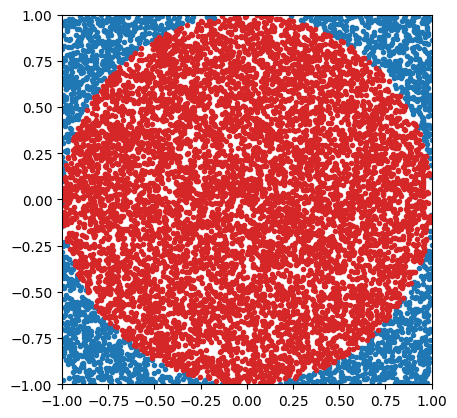
Imagine you’re throwing darts, and you’re not very accurate. You are trying to hit a spot somewhere within a circular target, but you can’t manage to do much better than throw it somewhere within the square that bounds the target, hitting any point within the square with equal probability. The red dots are those darts that manage to hit the circle, and the blue dots are those darts that don’t.

%matplotlib inline
import pylab as plt

x, y = np.random.uniform(-1, 1, (2, 10_000))
ind = x ** 2 + y ** 2 <= 1
plt.subplot(111, aspect='equal')
plt.plot(x[~ind], y[~ind], '.', rasterized=True)
plt.plot(x[ind], y[ind], '.', color='C3', rasterized=True)
plt.xlim(-1, 1)
plt.ylim(-1, 1);

../../_images/dcccd32936eedfd89feecc7ea55cdee560c4f7d669b9dcd3e3beee8fd4056815.png

The following code is a pure Python implementation to calculate an approximation of \(\pi\).

import random
import numpy as np


@timeit
def monte_carlo_pi_part(n: int) -> int:
    """ Calculate the number np points out of n attempts in the unit circle """
    count = 0
    for i in range(n):
        x = random.random()
        y = random.random()

        # if it is within the unit circle
        if x * x + y * y <= 1:
            count = count + 1

    return count

# Nummber of points to use for the Pi estimation
n = 10_000_000
estimate = monte_carlo_pi_part(n) / (n * 1.0) * 4

error = np.pi - estimate

print(f"Estimated value of Pi:: {estimate:g}")
print(f"               error :: {error:e}")

Timing  monte_carlo_pi_part   :  2.379375696182251  seconds
Estimated value of Pi:: 3.14143
               error :: 1.666536e-04

Rewrite the above code to optimize the speed. You can use numpy, Cython or else.

Numpy version

Timing  new_monte_carlo_pi_part   :  0.15527892112731934  seconds
Estimated value of Pi:: 3.14154
               error :: 5.505359e-05
speed up:  15.323236913987229

Cython version

# Nummber of points to use for the Pi estimation
new_monte_carlo_pi_part = timeit(new_monte_carlo_pi_part)

estimate = new_monte_carlo_pi_part(n) / (n * 1.0) * 4

error = np.pi - estimate

print(f"Estimated value of Pi:: {estimate:g}")
print(f"               error :: {error:e}")

print("speed up: ", monte_carlo_pi_part.last_execution_time[0] / new_monte_carlo_pi_part.last_execution_time[0])

Timing  new_monte_carlo_pi_part   :  0.12908673286437988  seconds
Estimated value of Pi:: 3.14113
               error :: 4.622536e-04
speed up:  18.4323798688286

# cleaning up
!rm -f mprun_demo.py

Optimizing Scientific Python codes

Contents

Optimizing Scientific Python codes#

Advanced debugging#

pdb, the Python debugger#

Navigating the Code#

Viewing and Changing Data#

Getting Help and Exiting#

IPython %xmode#

Defensive programming#

Unit tests in scientific computing#

The basics#

A good test is divided in three parts:#

Tips#

Numerical traps to avoid#

Testing learning algorithm#

Good practice: Test-driven development (TDD)#

Optimization and Profiling#

What is the strategy to optimize codes?#

Some simple examples#

Using timeit#

Profiling code, cProfile#

Line-by-Line Profiling with %lprun#

Profiling Memory Use: %memit and `%mprun``#

IPython tools#

Optimizing loops#

Python vs. Numpy vs. Cython#

Exercise: calulating \(\pi\)#

`pdb`, the Python debugger#

IPython `%xmode`#

Line-by-Line Profiling with `%lprun`#

Profiling Memory Use: `%memit` and `%mprun``#